SVM Kernels Explained: How to Tackle Nonlinear Data in Machine Learning
SVM Kernels Explained: How to Tackle Nonlinear Data in Machine Learning 관련

Have you ever considered how your phone can recognize handwritten text and convert it into regular computer text? Or how your email can separate messages automatically into spam and non-spam categories?
Both of these examples work based on classification tasks, as does the facial recognition feature on your phone.
When building a classification algorithm, real-world data often has a non-linear relationship. And many machine learning classification algorithms struggle with non-linear algorithms. But in this article, we'll be looking at how Support Vector Machine (SVM) kernel functions can help to solve this problem. We’ll go in-depth into a Python implementation of non-linear classification and SVM kernel functions.
Prerequisites
Overview of the Support Vector Machine (SVM) Technique
Support Vector Machine (SVM) is a supervised learning algorithm. It uses a hyperplane that divides features inside a feature space into distinct categories. It’s effective for both classification and regression applications.
By identifying the optimal dividing line or plane that will serve as the decision boundary, SVM seeks to maximize the margin between the various target variables. It’s primarily utilized in classification tasks and is very helpful in ignoring outliers. It categorizes the data points of the features in the dataset into distinct outputs or classes.
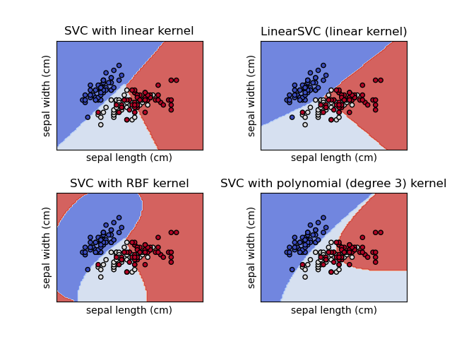
SVM seeks to achieve the optimal maximum margin and an ideal or near-perfect separation. There are various applications for SVM, such as image classification, face detection, text classification, image classification, and bioinformatics. SVM is also efficient in linear and non-linear classification problems.
Importance of Kernel methods in SVM
Nonlinear classification is a sort of classification that involves categorizing features that have non-linear, curved, or complex decision boundaries. Decision boundaries are regions of space that separate two different classes.
In linear classification tasks, the region of space between the different classes such as if the email is spam or not can be easily separated with a straight line. But in non-linear relationships, it could have a circular, parabola, or a complex-shape decision boundary.
Non-linear classification tasks have patterns that cannot be discovered by linear models. This is because the features have a non-linear relationship with each other.
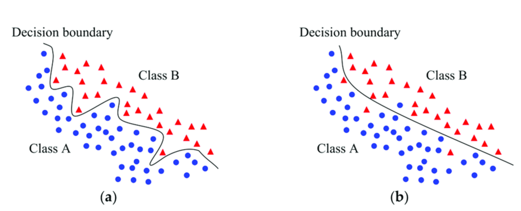
SVM as a linear classification algorithm isn’t efficient for a non-linear data. To handle this sort of data, it will require a kernel method, which is the core topic of this article.
A kernel method is a technique used in SVM to transform non-linear data into higher dimensions. For example, if the data has a complex decision boundary in a 2-Dimensional space (as I’ll explain further in the later part of this article), it can be transformed into a 3-Dimensional space. This allows efficient classification just with a linear plane.
The goal of the article is to teach you about SVM kernels and their application to non-linear classification tasks.
Fundamentals of SVM
Linear Classifiers and Margin Maximization
Linear classifiers are classification algorithms that make predictions by using a straight line of best fit as a decision boundary between two or more categories.
Marginal planes are used to determine the support vector in the classification task. Support vectors are the data points in the dataset that are used to separate the different target variable categories - they are data points very close to the decision boundary.
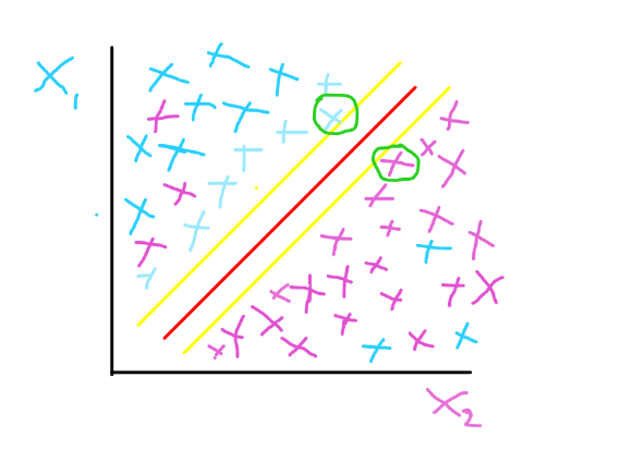
In the image below, the marginal planes are the yellow lines, while the hyperplane is the red line. The hyperplane serves as the line of best fit or decision boundary. The data points that are closest to the marginal plane are the support vectors - the data points encircled in green in the image below.
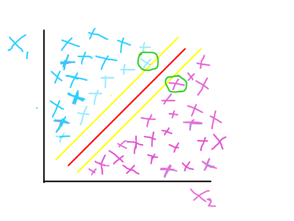
The marginal plane aims to achieve a maximum margin between its plane and the hyperplane - both having equal distance from hyperplane to achieve the best classification. The hyperplane in the image above shows a perfect linear relationship between feature x1 and feature x2. The support vectors also help to establish the location of the marginal plane.
We have the hard margin and the soft margin, serving as model optimization methodologies for the SVM. The hard margin shows that you cannot find a data point of feature x1 in the same area where there are feature x2 data points and vice versa. It used to describe a perfect classification by the algorithm. The image above gives a representation of a hard margin.
A soft margin shows that the classification is imperfect, because you can find some data points of feature x1 in the same area where we have data points of feature two, which could be caused by outliers. The image below gives a representation of soft margin.
SVM Objective Function
For a binary classification, such as a dog or a cat, the dog can be represented as class and cat as . This shows that the decision boundary or hyperplane is the determining factor. Any value above the plane is given as , and the class below the plane is given as . The mathematical function for the hyperplane is given as:
The variables used are:
- : Weight vector (defining the orientation of the hyperplane)
- : Bias term (defining the position of the hyperplane)
- : Input feature vector
The classification decision is based on the sign of
Hard Margin SVM
The Hard Margin SVM ensures all the data points are all properly classified without error, ensuring that the data points don’t find themselves in the other part of the hyperplane, and also maximizing the margin. It’s an effective method for a “noise-free” dataset. This is achieved by minimizing an objective function given below:
Hard Margin SVM Objective Function:
Subject to
Where:
- : Class label of the -th sample ( or )
- : Feature vector of the -th sample
This constraint given above in the objective function ensures that all the data points are not misclassified and the stay outside the margin.
Soft Margin SVM
The Soft Margin SVM is lenient, as it allows some misclassifications. It’s suitable for real-world datasets, which are noisy, and it handles non-linearly separable data. It introduces a slack variable that penalizes incorrect predictions.
Objective Function:
Subject to:
Where:
- : Slack variables representing the degree of misclassification ormargin violation.
- : Regularization parameter controlling the trade-off betweenmargin maximization and error minimization.
The hyperparameter C helps to control the penalty for a balance between margin maximization and error minimization. A large C value minimizes the classification errors, but causes a smaller margin. A small C value allows some misclassifications but causes a larger margin.
Nonlinear Classification Problems
Non-linear classification problems include datasets with non-linear patterns that are difficult for linear SVM models to capture.
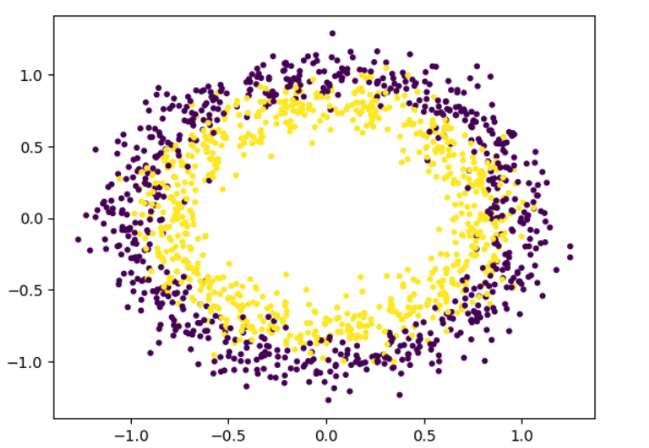
Non-linear classification contains datasets with complicated relationships and linear models like linear regression will not be able to accurately generate predictions or identify trends.
Understanding Kernel Functions
In kernel functions, we transform the dataset used in the classification task into a higher dimensional feature space. This line of action enables the hyperplane (a linear decision boundary) to split the data as linearly separable data.
For example, if a dataset contains three features in a 2D plane, the kernel function converts the data to a 3D plane, making it much simpler to partition the dataset using a basic hyperplane. This technique can be used to capture non-linear relationships in data.
To provide a clearer mental image, consider three distinct feature sets in the 2D plane (x and y). This can be taken to a 3D plane by the kernel machine, where features x1 and feature x2 may be in the x-y plane, which is readily divided by a simple hyperplane, and feature x3 may be in the y-z plane, which is already separated.
The Kernel Trick Explained
Transformation into a higher dimensional space is computationally intensive and is not the best option. But we know the importance of kernel functions in classifying non-linear data. So, what’s the way forward to still achieve the same feat while bypassing the cost of computation? It’s called the kernel trick. The kernel trick explains the “magic power” of the kernel functions.
The kernel trick is the computation of the inner or dot product between the data points in the original dimensional space instead of transforming the data into a higher-dimensional space before doing the computation.
The right side of the equation below shows the dot product of , representing the transformed vector into a higher dimensional space (which is not efficient). It’s the same as a kernel function at the left hand side:
The purpose of the kernel trick is to perform computation based on the data point in its original dimensional space, instead of performing calculations on complex data that might require an infinite number of dimensions.
Mathematical Implementation of the Kernel Trick
Suppose we have two classes of data that are non-linear in the 2D space representing the original feature space. No straight line can separate these points because they lie diagonally across the origin.
The 2D data is given as:
Let's use a mapping function:
Mapping and :
Dot Product in Higher-Dimensional Space:
This is the dot product of and after explicitlymapping them to the higher-dimensional space.
Polynomial Kernel Definition:
For this example:
Given:
Compute :
Using the kernel trick, we directly compute the dot product in the higherdimensional space without explicitly mapping the points.
Popular Kernel Functions
For a dataset that is linearly separable, the linear kernel is ideal. When used for non-linear data sets, which are the main topic of this article, it may result in underfitting and create a linear decision boundary. It’s provided as the input feature vectors' dot product.
This kernel merely constructs the hyperplane or line of best fit to divide the data points. It does not perform any particular transformation to a higher dimension.
The polynomial kernel transforms the data into a polynomial feature space of order d. It does a dot product on the feature vector with a constant c, all within the degree of d. The higher the degree of the polynomial, the better the kernel captures the relationships in the nonlinear dataset.
The Gaussian kernel, also known as the RBF kernel, is often used in SVM to map the input feature vector to an infinite-dimensional feature space using a Gaussian function. This kernel can handle more complex relationships.
The sigmoid kernel acts similarly to the activation function in neural networks. It functions similarly to a two-layered perception network and can map data into a higher-dimensional feature space.
There are other kernel functions such as Laplacian kernels, hyperbolic kernels, exponential kernels, and custom kernels that you can look into if you’re curious.
How to Choose the Right Kernel
The various kernel functions are applied based on the linear and nonlinear relationships in the feature space. The linear kernel is simple and fast, and it works well with linearly separable data but not with high-dimensional data.
The polynomial kernel is well-suited for data with non-linear or polynomial relationships, as well as low-dimensional data. The RBF kernel is ideal for dense data that you have no prior knowledge of. Finally, the sigmoid kernel works well for binary and categorical data points.
SVM Kernel Implementation
Let’s now go through an example showing how you can use this technique.
Step 1: Import the necessary libraries
import numpy as np
import matplotlib.pyplot as plt
from sklearn.datasets import make_circles
from mpl_toolkits.mplot3d import Axes3D
from sklearn.preprocessing import StandardScaler
Step 2: Generate the non-linear dataset
The non-linear dataset used in this article is a circle dataset from sklearn.datasets. We used 1500 samples with a random_state of 46 to keep the dataset consistent for reproducibility. We added a Gaussian noise to the data of 10%. This function generate_circle_data is implemented to generate the dataset used in the article.
def generate_circle_data(n_samples=1500, noise=0.10, random_state=46):
    """
    Generate two concentric circles dataset.

    Parameters:
    -----------
    n_samples : int
        The total number of points generated
    noise : float
        Standard deviation of Gaussian noise added to the data
    random_state : int
        Random seed for reproducibility

    Returns:
    --------
    X : array of shape [n_samples, 2]
        The generated samples
    y : array of shape [n_samples]
        The integer labels (0 or 1) for class membership of each sample
    """
    return make_circles(n_samples=n_samples,
                       noise=noise,
                       random_state=random_state)
Step 3: Plot the 2D Data
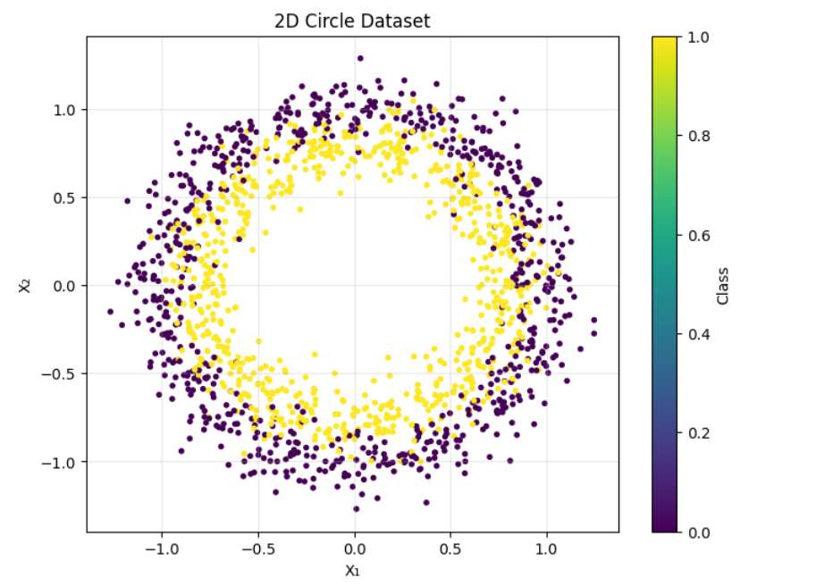
The data generated above comes in 2D form. Each color represents the two different data samples. The data points were plotted which allows us to see it as a circular dataset using the Matplotlib library.
def plot_2d_data(X, y, title="2D Circle Dataset"):
    """
    Plot the 2D dataset with different colors for each class.

    Parameters:
    -----------
    X : array-like of shape (n_samples, 2)
        The input samples
    y : array-like of shape (n_samples,)
        The target values (class labels)
    title : str
        The title of the plot
    """
    plt.figure(figsize=(8, 6))
    plt.scatter(X[:, 0], X[:, 1], c=y, marker='.', cmap='viridis')
    plt.title(title)
    plt.xlabel('X₁')
    plt.ylabel('X₂')
    plt.colorbar(label='Class')
    plt.grid(True, alpha=0.3)
    plt.show()
The output image of the dataset is given below:
Step 4: Transform into a Higher-Dimensional Space
The data in 2D is transformed into a 3D space using the polynomial kernel. We achieved this by creating a third feature X3 so it can be mapped into a higher dimensional space for easy separation.
def transform_to_3d(X):
    """Transform 2D data to 3D using radius-based transformation"""
    X1 = X[:, 0].reshape(-1, 1)
    X2 = X[:, 1].reshape(-1, 1)
    # Modified transformation to create better separation
    X3 = X1**2 + X2**2
    return np.hstack((X1, X2, X3))
Step 5: Plot the 3D Transformation
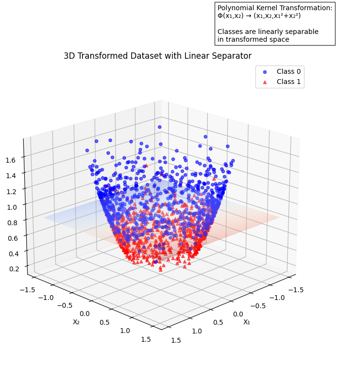
The next step is to plot the 3D transformed dataset. It now looks like a U-shaped bowl, and is separated with a hyperplane after fitting a LinearSVC model from the sklearn library as the kernel we’re using. This shows a practical example of the concepts you’ve learned so far:
def plot_3d_transformation_with_separator(X_transformed, y, title="3D Transformed Dataset with Linear Separator"):
    """Plot the 3D transformed dataset with a clear linear separating plane"""

    # Scale the transformed features
    scaler = StandardScaler()
    X_scaled = scaler.fit_transform(X_transformed)

    # Fit linear SVM with adjusted parameters for better separation
    svm = LinearSVC(C=1.0, dual="auto", max_iter=5000)
    svm.fit(X_scaled, y)

    # Create the 3D plot
    fig = plt.figure(figsize=(12, 8))
    ax = fig.add_subplot(111, projection='3d')

    # Plot the two classes with different colors and markers for clarity
    class_0 = y == 0
    class_1 = y == 1

    ax.scatter(X_transformed[class_0, 0],
              X_transformed[class_0, 1],
              X_transformed[class_0, 2],
              c='blue',
              marker='o',
              label='Class 0',
              alpha=0.6)

    ax.scatter(X_transformed[class_1, 0],
              X_transformed[class_1, 1],
              X_transformed[class_1, 2],
              c='red',
              marker='^',
              label='Class 1',
              alpha=0.6)

    # Create a grid for the separator plane
    x_min, x_max = X_transformed[:, 0].min() - 0.2, X_transformed[:, 0].max() + 0.2
    y_min, y_max = X_transformed[:, 1].min() - 0.2, X_transformed[:, 1].max() + 0.2

    xx, yy = np.meshgrid(np.linspace(x_min, x_max, 50),
                        np.linspace(y_min, y_max, 50))

    # Get the separating plane coefficients
    w = svm.coef_[0]
    b = svm.intercept_[0]

    # Calculate z coordinates of the plane
    grid_points = np.c_[xx.ravel(), yy.ravel(), np.zeros(xx.ravel().shape[0])]
    scaled_grid = scaler.transform(grid_points)

    # Calculate the separator plane
    z = (-w[0] * scaled_grid[:, 0] - w[1] * scaled_grid[:, 1] - b) / w[2]
    z = z.reshape(xx.shape)
    z = scaler.inverse_transform(np.c_[xx.ravel(), yy.ravel(), z.ravel()])[:, 2].reshape(xx.shape)

    # Plot the separating plane with adjusted transparency
    surface = ax.plot_surface(xx, yy, z, alpha=0.3, cmap='coolwarm')

    # Customize the plot
    ax.set_xlabel('X₁')
    ax.set_ylabel('X₂')
    ax.set_zlabel('X₁² + X₂²')
    ax.set_title(title)

    # Add legend
    ax.legend()

    # Adjust the viewing angle for better visualization
    ax.view_init(elev=20, azim=45)

    # Add text description
    ax.text2D(0.05, 0.95,
              "Polynomial Kernel Transformation:\n\phi\left(x₁,x₂) → (x₁,x₂,x₁²+x₂²)\n\nClasses are linearly separable\nin transformed space",
              transform=ax.transAxes,
              bbox=dict(facecolor='white', alpha=0.8))

    plt.show()

def main():
    # Generate and plot the dataset
    X, y = generate_circle_data()

    # Transform and plot 3D data with clear separator
    X_transformed = transform_to_3d(X)
    plot_3d_transformation_with_separator(X_transformed, y)

if __name__ == "__main__":
    main()
The main function is a function of functions that put together all the other functions such as generate_circle_data, transform_to_3d and plot_3d_transformation_with_separator together to establish the model.
Here’s the full code
import numpy as np
import matplotlib.pyplot as plt
from sklearn.datasets import make_circles
from mpl_toolkits.mplot3d import Axes3D
from sklearn.preprocessing import StandardScaler

def generate_circle_data(n_samples=1500, noise=0.10, random_state=46):
    """
    Generate two concentric circles dataset.

    Parameters:
    -----------
    n_samples : int
        The total number of points generated
    noise : float
        Standard deviation of Gaussian noise added to the data
    random_state : int
        Random seed for reproducibility

    Returns:
    --------
    X : array of shape [n_samples, 2]
        The generated samples
    y : array of shape [n_samples]
        The integer labels (0 or 1) for class membership of each sample
    """
    return make_circles(n_samples=n_samples,
                       noise=noise,
                       random_state=random_state)

def plot_2d_data(X, y, title="2D Circle Dataset"):
    """
    Plot the 2D dataset with different colors for each class.

    Parameters:
    -----------
    X : array-like of shape (n_samples, 2)
        The input samples
    y : array-like of shape (n_samples,)
        The target values (class labels)
    title : str
        The title of the plot
    """
    plt.figure(figsize=(8, 6))
    plt.scatter(X[:, 0], X[:, 1], c=y, marker='.', cmap='viridis')
    plt.title(title)
    plt.xlabel('X₁')
    plt.ylabel('X₂')
    plt.colorbar(label='Class')
    plt.grid(True, alpha=0.3)
    plt.show()

def transform_to_3d(X):
    """Transform 2D data to 3D using radius-based transformation"""
    X1 = X[:, 0].reshape(-1, 1)
    X2 = X[:, 1].reshape(-1, 1)
    # Modified transformation to create better separation
    X3 = X1**2 + X2**2
    return np.hstack((X1, X2, X3))

def plot_3d_transformation_with_separator(X_transformed, y, title="3D Transformed Dataset with Linear Separator"):
    """Plot the 3D transformed dataset with a clear linear separating plane"""

    # Scale the transformed features
    scaler = StandardScaler()
    X_scaled = scaler.fit_transform(X_transformed)

    # Fit linear SVM with adjusted parameters for better separation
    svm = LinearSVC(C=1.0, dual="auto", max_iter=5000)
    svm.fit(X_scaled, y)

    # Create the 3D plot
    fig = plt.figure(figsize=(12, 8))
    ax = fig.add_subplot(111, projection='3d')

    # Plot the two classes with different colors and markers for clarity
    class_0 = y == 0
    class_1 = y == 1

    ax.scatter(X_transformed[class_0, 0],
              X_transformed[class_0, 1],
              X_transformed[class_0, 2],
              c='blue',
              marker='o',
              label='Class 0',
              alpha=0.6)

    ax.scatter(X_transformed[class_1, 0],
              X_transformed[class_1, 1],
              X_transformed[class_1, 2],
              c='red',
              marker='^',
              label='Class 1',
              alpha=0.6)

    # Create a grid for the separator plane
    x_min, x_max = X_transformed[:, 0].min() - 0.2, X_transformed[:, 0].max() + 0.2
    y_min, y_max = X_transformed[:, 1].min() - 0.2, X_transformed[:, 1].max() + 0.2

    xx, yy = np.meshgrid(np.linspace(x_min, x_max, 50),
                        np.linspace(y_min, y_max, 50))

    # Get the separating plane coefficients
    w = svm.coef_[0]
    b = svm.intercept_[0]

    # Calculate z coordinates of the plane
    grid_points = np.c_[xx.ravel(), yy.ravel(), np.zeros(xx.ravel().shape[0])]
    scaled_grid = scaler.transform(grid_points)

    # Calculate the separator plane
    z = (-w[0] * scaled_grid[:, 0] - w[1] * scaled_grid[:, 1] - b) / w[2]
    z = z.reshape(xx.shape)
    z = scaler.inverse_transform(np.c_[xx.ravel(), yy.ravel(), z.ravel()])[:, 2].reshape(xx.shape)

    # Plot the separating plane with adjusted transparency
    surface = ax.plot_surface(xx, yy, z, alpha=0.3, cmap='coolwarm')

    # Customize the plot
    ax.set_xlabel('X₁')
    ax.set_ylabel('X₂')
    ax.set_zlabel('X₁² + X₂²')
    ax.set_title(title)

    # Add legend
    ax.legend()

    # Adjust the viewing angle for better visualization
    ax.view_init(elev=20, azim=45)

    # Add text description
    ax.text2D(0.7, 1.07,
              "Polynomial Kernel Transformation:\nΦ(x₁,x₂) → (x₁,x₂,x₁²+x₂²)\n\nClasses are linearly separable\nin transformed space",
              transform=ax.transAxes,
              bbox=dict(facecolor='white', alpha=0.8))

    plt.show()

def main():
    # Generate and plot the dataset
    X, y = generate_circle_data()

    # Transform and plot 3D data with clear separator
    X_transformed = transform_to_3d(X)
    plot_3d_transformation_with_separator(X_transformed, y)

if __name__ == "__main__":
    main()
Conclusion
In this article, you learned about the efficiency of SVM kernels for non-linear classification applications. The various functions demonstrated computational efficiency by changing input data into higher dimensional data, as shown in the example, without requiring vast amounts of storage or processing.
SVM can be used in a variety of classification tasks, including image and text classification, and it has proven to be extremely efficient.
References