The Bubble Sort Algorithm in Python

Santiago ValdarramaApril 15, 2020About 5 min

The Bubble Sort Algorithm in Python 관련

In this tutorial, you'll learn all about five different sorting algorithms in Python from both a theoretical and a practical standpoint. You'll also learn several related and important concepts, including Big O notation and recursion.

Sorting Algorithms in Python

Bubble Sort is one of the most straightforward sorting algorithms. Its name comes from the way the algorithm works: With every new pass, the largest element in the list “bubbles up” toward its correct position.

Bubble sort consists of making multiple passes through a list, comparing elements one by one, and swapping adjacent items that are out of order.

Implementing Bubble Sort in Python

Here’s an implementation of a bubble sort algorithm in Python:

def bubble_sort(array):
    n = len(array)

    for i in range(n):
        # Create a flag that will allow the function to
        # terminate early if there's nothing left to sort
        already_sorted = True

        # Start looking at each item of the list one by one,
        # comparing it with its adjacent value. With each
        # iteration, the portion of the array that you look at
        # shrinks because the remaining items have already been
        # sorted.
        for j in range(n - i - 1):
            if array[j] > array[j + 1]:
                # If the item you're looking at is greater than its
                # adjacent value, then swap them
                array[j], array[j + 1] = array[j + 1], array[j]

                # Since you had to swap two elements,
                # set the `already_sorted` flag to `False` so the
                # algorithm doesn't finish prematurely
                already_sorted = False

        # If there were no swaps during the last iteration,
        # the array is already sorted, and you can terminate
        if already_sorted:
            break

    return array

Since this implementation sorts the array in ascending order, each step “bubbles” the largest element to the end of the array. This means that each iteration takes fewer steps than the previous iteration because a continuously larger portion of the array is sorted.

The loops in lines 4 and 10 determine the way the algorithm runs through the list. Notice how j initially goes from the first element in the list to the element immediately before the last. During the second iteration, j runs until two items from the last, then three items from the last, and so on. At the end of each iteration, the end portion of the list will be sorted.

As the loops progress, line 15 compares each element with its adjacent value, and line 18 swaps them if they are in the incorrect order. This ensures a sorted list at the end of the function.

Note

The already_sorted flag in lines 13, 23, and 27 of the code above is an optimization to the algorithm, and it’s not required in a fully functional bubble sort implementation. However, it allows the function to skip unnecessary steps if the list ends up wholly sorted before the loops have finished.

As an exercise, you can remove the use of this flag and compare the runtimes of both implementations.

To properly analyze how the algorithm works, consider a list with values [8, 2, 6, 4, 5]. Assume you’re using bubble_sort() from above. Here’s a figure illustrating what the array looks like at each iteration of the algorithm:

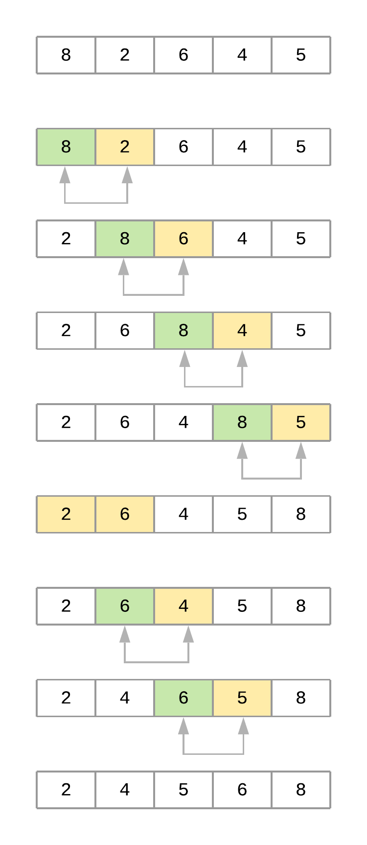
Now take a step-by-step look at what’s happening with the array as the algorithm progresses:

The code starts by comparing the first element, 8, with its adjacent element, 2. Since $8>2$ , the values are swapped, resulting in the following order: [2, 8, 6, 4, 5].
The algorithm then compares the second element, 8, with its adjacent element, 6. Since $8>6$ , the values are swapped, resulting in the following order: [2, 6, 8, 4, 5].
Next, the algorithm compares the third element, 8, with its adjacent element, 4. Since $8>4$ , it swaps the values as well, resulting in the following order: [2, 6, 4, 8, 5].
Finally, the algorithm compares the fourth element, 8, with its adjacent element, 5, and swaps them as well, resulting in [2, 6, 4, 5, 8]. At this point, the algorithm completed the first pass through the list ( $i=0$ ). Notice how the value 8 bubbled up from its initial location to its correct position at the end of the list.
The second pass ( $i=1$ ) takes into account that the last element of the list is already positioned and focuses on the remaining four elements, [2, 6, 4, 5]. At the end of this pass, the value 6 finds its correct position. The third pass through the list positions the value 5, and so on until the list is sorted.

Measuring Bubble Sort’s Big O Runtime Complexity

Your implementation of bubble sort consists of two nested for loops in which the algorithm performs $n-1$ comparisons, then $n-2$ comparisons, and so on until the final comparison is done. This comes at a total of $\left(n-1\right)+\left(n-2\right)+\left(n-3\right)+\ldots+2+1= \frac{n\left(n-1\right)}{2}$ comparisons, which can also be written as $\frac{1}{2}n^{2}-\frac{1}{2}n$ .

You learned earlier that Big O focuses on how the runtime grows in comparison to the size of the input. That means that, in order to turn the above equation into the Big O complexity of the algorithm, you need to remove the constants because they don’t change with the input size.

Doing so simplifies the notation to $n^{2}-n$ . Since $n^{2}$ grows much faster than $n$ , this last term can be dropped as well, leaving bubble sort with an average- and worst-case complexity of $O\left(n^{2}\right)$ .

In cases where the algorithm receives an array that’s already sorted—and assuming the implementation includes the already_sorted flag optimization explained before—the runtime complexity will come down to a much better $O\left(n\right)$ because the algorithm will not need to visit any element more than once.

$O\left(n\right)$ , then, is the best-case runtime complexity of bubble sort. But keep in mind that best cases are an exception, and you should focus on the average case when comparing different algorithms.

Timing Your Bubble Sort Implementation

Using your run_sorting_algorithm() from earlier in this tutorial, here’s the time it takes for bubble sort to process an array with ten thousand items. Line 8 replaces the name of the algorithm and everything else stays the same:

if __name__ == "__main__":
    # Generate an array of `ARRAY_LENGTH` items consisting
    # of random integer values between 0 and 999
    array = [randint(0, 1000) for i in range(ARRAY_LENGTH)]

    # Call the function using the name of the sorting algorithm
    # and the array you just created
    run_sorting_algorithm(algorithm="bubble_sort", array=array)

You can now run the script to get the execution time of bubble_sort:

python sorting.py
#
# Algorithm: bubble_sort. Minimum execution time: 73.21720498399998

It took 73 seconds to sort the array with ten thousand elements. This represents the fastest execution out of the ten repetitions that run_sorting_algorithm() runs. Executing this script multiple times will produce similar results.

Note

A single execution of bubble sort took 73 seconds, but the algorithm ran ten times using timeit.repeat(). This means that you should expect your code to take around $73\times10=730$ seconds to run, assuming you have similar hardware characteristics. Slower machines may take much longer to finish.

Analyzing the Strengths and Weaknesses of Bubble Sort

The main advantage of the bubble sort algorithm is its simplicity. It is straightforward to both implement and understand. This is probably the main reason why most computer science courses introduce the topic of sorting using bubble sort.

As you saw before, the disadvantage of bubble sort is that it is slow, with a runtime complexity of $O\left(n^{2}\right)$ . Unfortunately, this rules it out as a practical candidate for sorting large arrays.