The Merge Sort Algorithm in Python

Santiago ValdarramaApril 15, 2020About 6 min

The Merge Sort Algorithm in Python 관련

In this tutorial, you'll learn all about five different sorting algorithms in Python from both a theoretical and a practical standpoint. You'll also learn several related and important concepts, including Big O notation and recursion.

Sorting Algorithms in Python

Merge sort is a very efficient sorting algorithm. It’s based on the divide-and-conquer approach, a powerful algorithmic technique used to solve complex problems.

To properly understand divide and conquer, you should first understand the concept of recursion. Recursion involves breaking a problem down into smaller subproblems until they’re small enough to manage. In programming, recursion is usually expressed by a function calling itself.

Note

This tutorial doesn’t explore recursion in depth. To better understand how recursion works and see it in action using Python, check out Thinking Recursively in Python and Recursion in Python: An Introduction.

Divide-and-conquer algorithms typically follow the same structure:

The original input is broken into several parts, each one representing a subproblem that’s similar to the original but simpler.
Each subproblem is solved recursively.
The solutions to all the subproblems are combined into a single overall solution.

In the case of merge sort, the divide-and-conquer approach divides the set of input values into two equal-sized parts, sorts each half recursively, and finally merges these two sorted parts into a single sorted list.

Implementing Merge Sort in Python

The implementation of the merge sort algorithm needs two different pieces:

A function that recursively splits the input in half
A function that merges both halves, producing a sorted array

Here’s the code to merge two different arrays:

def merge(left, right):
    # If the first array is empty, then nothing needs
    # to be merged, and you can return the second array as the result
    if len(left) == 0:
        return right

    # If the second array is empty, then nothing needs
    # to be merged, and you can return the first array as the result
    if len(right) == 0:
        return left

    result = []
    index_left = index_right = 0

    # Now go through both arrays until all the elements
    # make it into the resultant array
    while len(result) < len(left) + len(right):
        # The elements need to be sorted to add them to the
        # resultant array, so you need to decide whether to get
        # the next element from the first or the second array
        if left[index_left] <= right[index_right]:
            result.append(left[index_left])
            index_left += 1
        else:
            result.append(right[index_right])
            index_right += 1

        # If you reach the end of either array, then you can
        # add the remaining elements from the other array to
        # the result and break the loop
        if index_right == len(right):
            result += left[index_left:]
            break

        if index_left == len(left):
            result += right[index_right:]
            break

    return result

merge() receives two different sorted arrays that need to be merged together. The process to accomplish this is straightforward:

Lines 4 and 9 check whether either of the arrays is empty. If one of them is, then there’s nothing to merge, so the function returns the other array.
Line 17 starts a while loop that ends whenever the result contains all the elements from both of the supplied arrays. The goal is to look into both arrays and combine their items to produce a sorted list.
Line 21 compares the elements at the head of both arrays, selects the smaller value, and appends it to the end of the resultant array.
Lines 31 and 35 append any remaining items to the result if all the elements from either of the arrays were already used.

With the above function in place, the only missing piece is a function that recursively splits the input array in half and uses merge() to produce the final result:

def merge_sort(array):
    # If the input array contains fewer than two elements,
    # then return it as the result of the function
    if len(array) < 2:
        return array

    midpoint = len(array) // 2

    # Sort the array by recursively splitting the input
    # into two equal halves, sorting each half and merging them
    # together into the final result
    return merge(
        left=merge_sort(array[:midpoint]),
        right=merge_sort(array[midpoint:]))

Here’s a quick summary of the code:

Line 44 acts as the stopping condition for the recursion. If the input array contains fewer than two elements, then the function returns the array. Notice that this condition could be triggered by receiving either a single item or an empty array. In both cases, there’s nothing left to sort, so the function should return.
Line 47 computes the middle point of the array.
Line 52 calls merge(), passing both sorted halves as the arrays.

Notice how this function calls itself recursively, halving the array each time. Each iteration deals with an ever-shrinking array until fewer than two elements remain, meaning there’s nothing left to sort. At this point, merge() takes over, merging the two halves and producing a sorted list.

Take a look at a representation of the steps that merge sort will take to sort the array [8, 2, 6, 4, 5]:

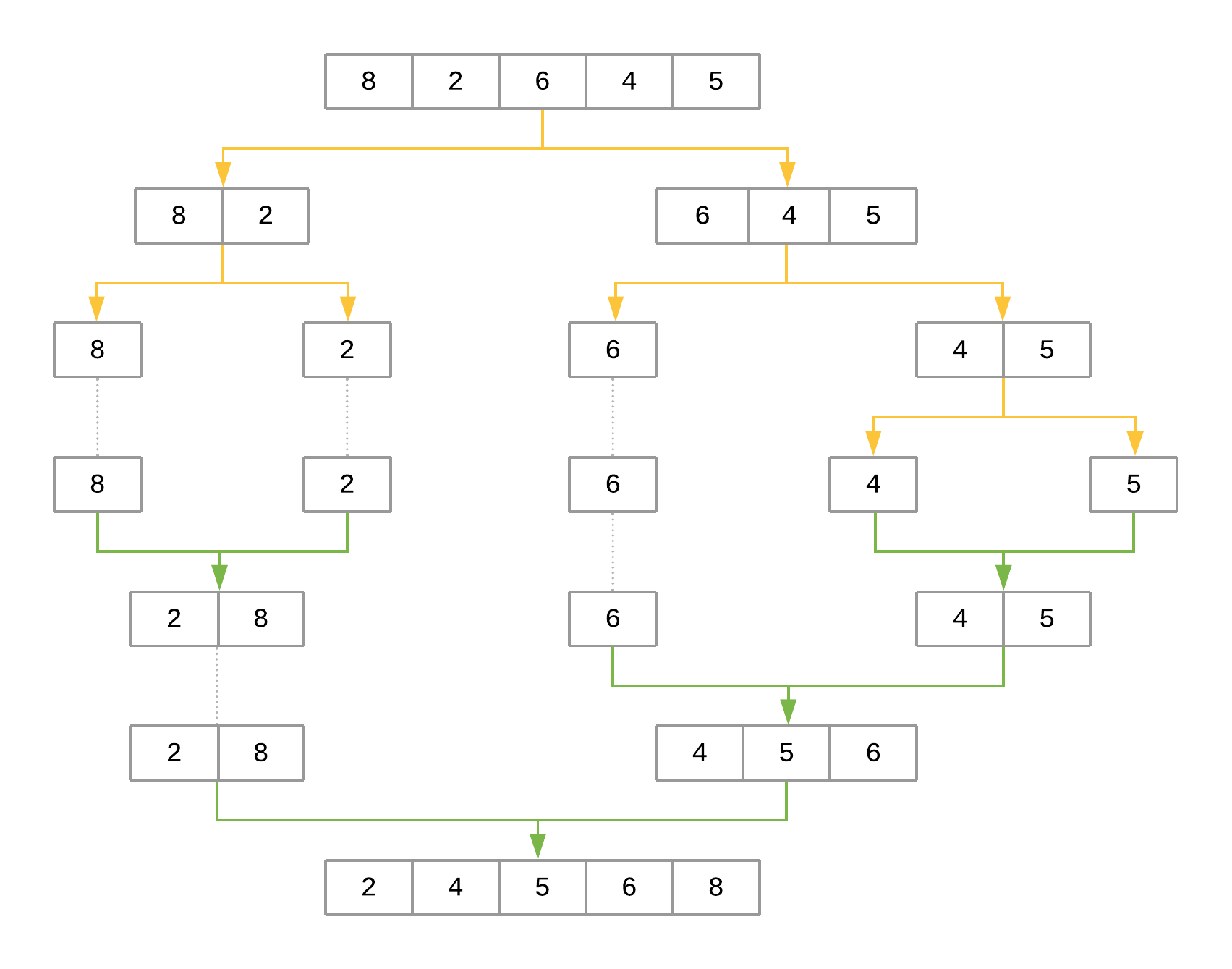
The figure uses yellow arrows to represent halving the array at each recursion level. The green arrows represent merging each subarray back together. The steps can be summarized as follows:

The first call to merge_sort() with [8, 2, 6, 4, 5] defines midpoint as 2. The midpoint is used to halve the input array into array[:2] and array[2:], producing [8, 2] and [6, 4, 5], respectively. merge_sort() is then recursively called for each half to sort them separately.
The call to merge_sort() with [8, 2] produces [8] and [2]. The process repeats for each of these halves.
The call to merge_sort() with [8] returns [8] since that’s the only element. The same happens with the call to merge_sort() with [2].
At this point, the function starts merging the subarrays back together using merge(), starting with [8] and [2] as input arrays, producing [2, 8] as the result.
On the other side, [6, 4, 5] is recursively broken down and merged using the same procedure, producing [4, 5, 6] as the result.
In the final step, [2, 8] and [4, 5, 6] are merged back together with merge(), producing the final result: [2, 4, 5, 6, 8].

Measuring Merge Sort’s Big O Complexity

To analyze the complexity of merge sort, you can look at its two steps separately:

merge() has a linear runtime. It receives two arrays whose combined length is at most $n$ (the length of the original input array), and it combines both arrays by looking at each element at most once. This leads to a runtime complexity of $O\left(n\right)$ .
The second step splits the input array recursively and calls merge() for each half. Since the array is halved until a single element remains, the total number of halving operations performed by this function is $\log_{2}{n}$ . Since merge() is called for each half, we get a total runtime of $O\left(n\:\log_{2}{n}\right)$ .

Interestingly, $O\left(n\:\log_{2}{n}\right)$ is the best possible worst-case runtime that can be achieved by a sorting algorithm.

Timing Your Merge Sort Implementation

To compare the speed of merge sort with the previous two implementations, you can use the same mechanism as before and replace the name of the algorithm in line 8:

if __name__ == "__main__":
    # Generate an array of `ARRAY_LENGTH` items consisting
    # of random integer values between 0 and 999
    array = [randint(0, 1000) for i in range(ARRAY_LENGTH)]

    # Call the function using the name of the sorting algorithm
    # and the array you just created
    run_sorting_algorithm(algorithm="merge_sort", array=array)

You can execute the script to get the execution time of merge_sort:

python sorting.py
# 
# Algorithm: merge_sort. Minimum execution time: 0.6195857160000173

Compared to bubble sort and insertion sort, the merge sort implementation is extremely fast, sorting the ten-thousand-element array in less than a second!

Analyzing the Strengths and Weaknesses of Merge Sort

Thanks to its runtime complexity of $O\left(n\:\log_{2}{n}\right)$ , merge sort is a very efficient algorithm that scales well as the size of the input array grows. It’s also straightforward to parallelize because it breaks the input array into chunks that can be distributed and processed in parallel if necessary.

That said, for small lists, the time cost of the recursion allows algorithms such as bubble sort and insertion sort to be faster. For example, running an experiment with a list of ten elements results in the following times:

Algorithm: bubble_sort. Minimum execution time: 0.000018774999999998654
Algorithm: insertion_sort. Minimum execution time: 0.000029786000000000395
Algorithm: merge_sort. Minimum execution time: 0.00016983000000000276

Both bubble sort and insertion sort beat merge sort when sorting a ten-element list.

Another drawback of merge sort is that it creates copies of the array when calling itself recursively. It also creates a new list inside merge() to sort and return both input halves. This makes merge sort use much more memory than bubble sort and insertion sort, which are both able to sort the list in place.

Due to this limitation, you may not want to use merge sort to sort large lists in memory-constrained hardware.