The Quicksort Algorithm in Python

Santiago ValdarramaApril 15, 2020About 6 min

The Quicksort Algorithm in Python 관련

In this tutorial, you'll learn all about five different sorting algorithms in Python from both a theoretical and a practical standpoint. You'll also learn several related and important concepts, including Big O notation and recursion.

Sorting Algorithms in Python

Just like merge sort, the Quicksort algorithm applies the divide-and-conquer principle to divide the input array into two lists, the first with small items and the second with large items. The algorithm then sorts both lists recursively until the resultant list is completely sorted.

Dividing the input list is referred to as partitioning the list. Quicksort first selects a pivot element and partitions the list around the pivot, putting every smaller element into a low array and every larger element into a high array.

Putting every element from the low list to the left of the pivot and every element from the high list to the right positions the pivot precisely where it needs to be in the final sorted list. This means that the function can now recursively apply the same procedure to low and then high until the entire list is sorted.

Implementing Quicksort in Python

Here’s a fairly compact implementation of Quicksort:

from random import randint

def quicksort(array):
    # If the input array contains fewer than two elements,
    # then return it as the result of the function
    if len(array) < 2:
        return array

    low, same, high = [], [], []

    # Select your `pivot` element randomly
    pivot = array[randint(0, len(array) - 1)]

    for item in array:
        # Elements that are smaller than the `pivot` go to
        # the `low` list. Elements that are larger than
        # `pivot` go to the `high` list. Elements that are
        # equal to `pivot` go to the `same` list.
        if item < pivot:
            low.append(item)
        elif item == pivot:
            same.append(item)
        elif item > pivot:
            high.append(item)

    # The final result combines the sorted `low` list
    # with the `same` list and the sorted `high` list
    return quicksort(low) + same + quicksort(high)

Here’s a summary of the code:

Line 6 stops the recursive function if the array contains fewer than two elements.
Line 12 selects the pivot element randomly from the list and proceeds to partition the list.
Lines 19 and 20 put every element that’s smaller than pivot into the list called low.
Lines 21 and 22 put every element that’s equal to pivot into the list called same.
Lines 23 and 24 put every element that’s larger than pivot into the list called high.
Line 28 recursively sorts the low and high lists and combines them along with the contents of the same list.

Here’s an illustration of the steps that Quicksort takes to sort the array [8, 2, 6, 4, 5]:

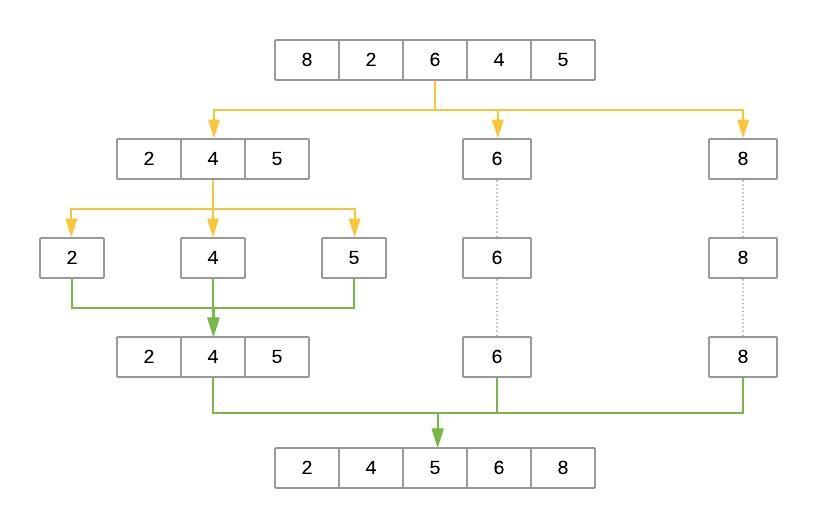
The yellow lines represent the partitioning of the array into three lists: low, same, and high. The green lines represent sorting and putting these lists back together. Here’s a brief explanation of the steps:

The pivot element is selected randomly. In this case, pivot is 6.
The first pass partitions the input array so that low contains [2, 4, 5], same contains [6], and high contains [8].
quicksort() is then called recursively with low as its input. This selects a random pivot and breaks the array into [2] as low, [4] as same, and [5] as high.
The process continues, but at this point, both low and high have fewer than two items each. This ends the recursion, and the function puts the array back together. Adding the sorted low and high to either side of the same list produces [2, 4, 5].
On the other side, the high list containing [8] has fewer than two elements, so the algorithm returns the sorted low array, which is now [2, 4, 5]. Merging it with same ([6]) and high ([8]) produces the final sorted list.

Selecting the `pivot` Element

Why does the implementation above select the pivot element randomly? Wouldn’t it be the same to consistently select the first or last element of the input list?

Because of how the Quicksort algorithm works, the number of recursion levels depends on where pivot ends up in each partition. In the best-case scenario, the algorithm consistently picks the median element as the pivot. That would make each generated subproblem exactly half the size of the previous problem, leading to at most $\log_{2}{n}$ levels.

On the other hand, if the algorithm consistently picks either the smallest or largest element of the array as the pivot, then the generated partitions will be as unequal as possible, leading to $n-1$ recursion levels. That would be the worst-case scenario for Quicksort.

As you can see, Quicksort’s efficiency often depends on the pivot selection. If the input array is unsorted, then using the first or last element as the pivot will work the same as a random element. But if the input array is sorted or almost sorted, using the first or last element as the pivot could lead to a worst-case scenario. Selecting the pivot at random makes it more likely Quicksort will select a value closer to the median and finish faster.

Another option for selecting the pivot is to find the median value of the array and force the algorithm to use it as the pivot. This can be done in $O\left(n\right)$ time. Although the process is little bit more involved, using the median value as the pivot for Quicksort guarantees you will have the best-case Big O scenario.

Measuring Quicksort’s Big O Complexity

With Quicksort, the input list is partitioned in linear time, $O\left(n\right)$ , and this process repeats recursively an average of $\log_{2}{n}$ times. This leads to a final complexity of $O\left(n\:\log_{2}{n}\right)$ .

That said, remember the discussion about how the selection of the pivot affects the runtime of the algorithm. The $O\left(n\right)$ best-case scenario happens when the selected pivot is close to the median of the array, and an $O\left(n^{2}\right)$ scenario happens when the pivot is the smallest or largest value of the array.

Theoretically, if the algorithm focuses first on finding the median value and then uses it as the pivot element, then the worst-case complexity will come down to $O\left(n\:\log_{2}{n}\right)$ . The median of an array can be found in linear time, and using it as the pivot guarantees the Quicksort portion of the code will perform in $O\left(n\:\log_{2}{n}\right)$ .

By using the median value as the pivot, you end up with a final runtime of $O\left(n\right)+O\left(n\:\log_{2}{n}\right)$ . You can simplify this down to $O\left(n\:\log_{2}{n}\right)$ because the logarithmic portion grows much faster than the linear portion.

Note

Although achieving $O\left(n\:\log_{2}{n}\right)$ is possible in Quicksort’s worst-case scenario, this approach is seldom used in practice. Lists have to be quite large for the implementation to be faster than a simple randomized selection of the pivot.

Randomly selecting the pivot makes the worst case very unlikely. That makes random pivot selection good enough for most implementations of the algorithm.

Timing Your Quicksort Implementation

By now, you’re familiar with the process for timing the runtime of the algorithm. Just change the name of the algorithm in line 8:

if __name__ == "__main__":
    # Generate an array of `ARRAY_LENGTH` items consisting
    # of random integer values between 0 and 999
    array = [randint(0, 1000) for i in range(ARRAY_LENGTH)]

    # Call the function using the name of the sorting algorithm
    # and the array you just created
    run_sorting_algorithm(algorithm="quicksort", array=array)

You can execute the script as you have before:

python sorting.py
#
# Algorithm: quicksort. Minimum execution time: 0.11675417600002902

Not only does Quicksort finish in less than one second, but it’s also much faster than merge sort (0.11 seconds versus 0.61 seconds). Increasing the number of elements specified by ARRAY_LENGTH from 10,000 to 1,000,000 and running the script again ends up with merge sort finishing in 97 seconds, whereas Quicksort sorts the list in a mere 10 seconds.

Analyzing the Strengths and Weaknesses of Quicksort

True to its name, Quicksort is very fast. Although its worst-case scenario is theoretically $O\left(n^{2}\right)$ , in practice, a good implementation of Quicksort beats most other sorting implementations. Also, just like merge sort, Quicksort is straightforward to parallelize.

One of Quicksort’s main disadvantages is the lack of a guarantee that it will achieve the average runtime complexity. Although worst-case scenarios are rare, certain applications can’t afford to risk poor performance, so they opt for algorithms that stay within $O\left(n\:\log_{2}{n}\right)$ regardless of the input.

Just like merge sort, Quicksort also trades off memory space for speed. This may become a limitation for sorting larger lists.

A quick experiment sorting a list of ten elements leads to the following results:

Algorithm: bubble_sort. Minimum execution time: 0.0000909000000000014
Algorithm: insertion_sort. Minimum execution time: 0.00006681900000000268
Algorithm: quicksort. Minimum execution time: 0.0001319930000000004

The results show that Quicksort also pays the price of recursion when the list is sufficiently small, taking longer to complete than both insertion sort and bubble sort.