Working With Jupyter Notebook in JupyterLab
Working With Jupyter Notebook in JupyterLab 관련

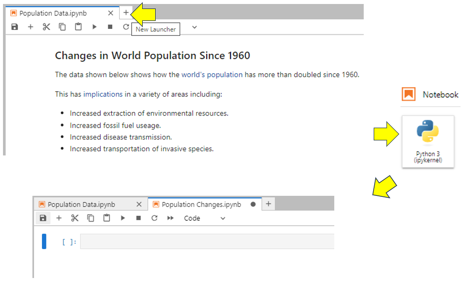
Although this tutorial isn't a dedicated Jupyter Notebook tutorial, you'll now perform some common tasks so you can appreciate what JupyterLab brings to Jupyter Notebooks. Start a new Jupyter Notebook within JupyterLab by clicking the large Python 3 button below the Notebook heading as shown:
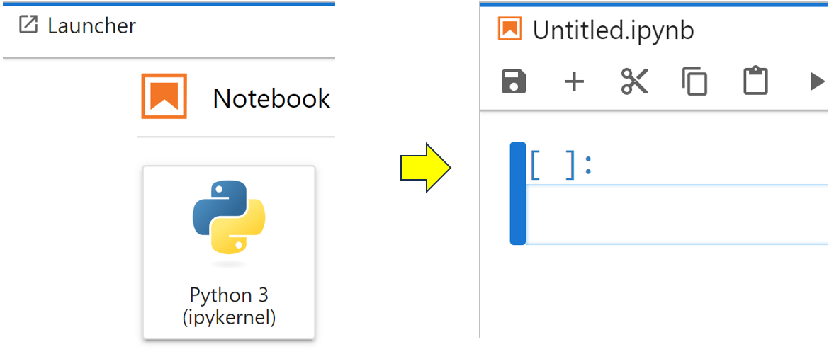
This will open a new Jupyter Notebook named Untitled.ipynb. You'll most likely want to give it a more descriptive name, and you can do so by right-clicking its tab, selecting Rename Notebook…, then changing the name to something more meaningful. In this example, you choose to rename it Population Data:
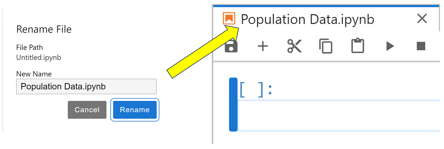
Once you've entered the new name, click the blue Rename button to update your notebook with its new name.
When you open a new notebook, it contains a single gray rectangle. This is a code cell as indicated by the Code text shown in a dropdown option of the toolbar above it. You won't be surprised to learn that this is where you enter program code, but you probably won't do this immediately. Usually, when you create a notebook, you'll want to start with some formatted Markdown text as an introduction.
To create some Markdown, select the code cell and then select Markdown from the dropdown menu in the toolbar. This will prepare the cell for you to enter Markdown text into. Now type the following Markdown text into this cell:
---
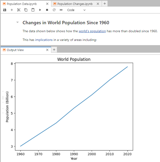
## Changes in World Population Since 1960
The data shown below shows how the
[world's population](https://worldometers.info/world-population/world-population-by-year/)
has more than doubled since 1960. This has [implications](https://ugc.berkeley.edu/background-content/population-growth/)
in a variety of areas including:
* Increased extraction of environmental resources.
* Increased fossil fuel usage.
* Increased disease transmission.
* Increased transportation of invasive species.
**The data below shows the population each decade since 1960:**
When you typed in the text, you may have wondered why you used the hashes, asterisks, and brackets. The best way to find out is to run the cell. You can do this either by clicking the small right-pointing triangle beneath the notebook's tab or by using Shift+Enter. Either way, you'll run the cell and render its Markdown on-screen:

As you can see, you used the # symbol to specify a heading, while your []() symbols created hyperlinks to the data sources. You created a bulleted list using single asterisks, while double asterisks made your text bold. In other words, you used these characters to define the format of your output.
If your Markdown cell didn't render correctly, then you can double-click on it and fix it. Rerun it once you've changed any errors, and it should render correctly. Remember, each symbol makes a significant difference as to how the result will look.
You may also have noticed that a fresh code cell has appeared below your Markdown cell. You then add in the following code:
decades = [1960, 1970, 1980, 1990, 2000, 2010, 2020]

# World population (billions)
population = [3, 3.7, 4.4, 5.3, 6.1, 7.0, 7.8]
You've entered the population data as two Python lists. Your first list contains decades, while the second contains the world's population for each decade. When you run the cell using Shift+Enter, the code runs and becomes formatted.
Although running this cell produces no output, running it is still important because it sets up the lists and assigns them to their variables. In other words, the notebook's kernel becomes aware of them, meaning the variables then become available to subsequent cells in your notebook, and even to other notebooks if you share this notebook's kernel.
While the data makes sense by itself, wouldn't it be more striking if you displayed it in a chart? Fortunately, you can do this by using the Matplotlib library. As with all third-party libraries, you need to install matplotlib into your Python environment because it's not part of the Python standard library.
The notebook interface allows you to install third-party packages into your current Python environment directly from a code cell, without needing to switch to a terminal. You can execute shell commands in a code cell by prefixing them with an exclamation point (!).
So, to install the matplotlib library, you type !python -m pip install matplotlib in a new code cell and run it. You'll know the code cell is running when a [*] appears next to it. This will change to a number in square brackets once the installation is finished. This number indicates the sequence in which that particular code cell was executed.
Once the command is complete, you'll see some installation output:
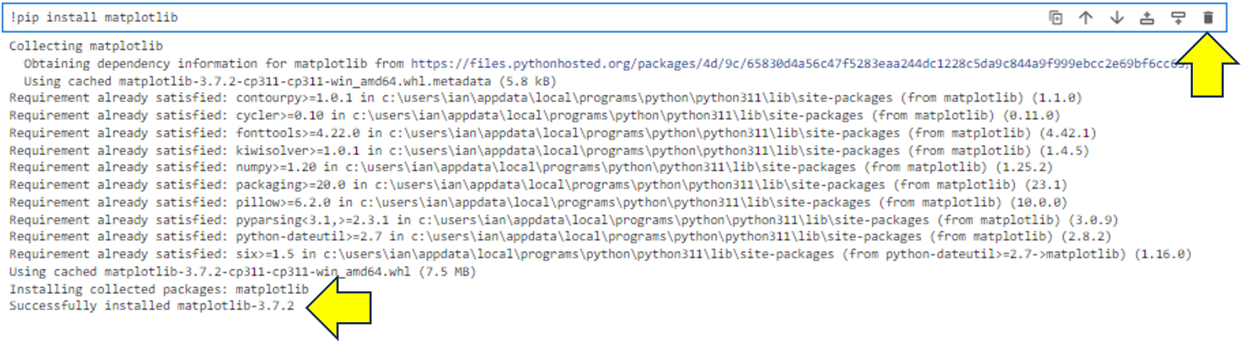
As you can see, a new code cell has appeared below the output of your pip command. You can verify that the installation was successful by reading the last line of output. You can then tidy up the notebook by selecting the cell containing the !python -m pip install matplotlib command and clicking the trash icon as shown. This will delete it. Don't worry, matplotlib will still be installed, and only the mess will be gone.
Note
You may have noticed the collection of icons to the left of the trash icon. These allow you to manipulate the cells. Hover your mouse over each of them to learn what they do. Feel free to click on any to clarify your understanding. You can also trash anything that you inadvertently create to get rid of it.
Now you display your data in a chart. To do this, type the following code into a new code cell and run it:
from matplotlib import pyplot as plt

plt.plot(decades, population)

plt.xlabel("Year")
plt.ylabel("Population (Billion)")
plt.title("World Population")

plt.show()
First of all, you import pyplot. This provides access to a set of functions that you use to manage your plots. For example, you create the basic plot using pyplot's plot() function. You also use functions to define the labels on each axis and to give your chart its title. When you type the above code into the new code cell and run it, you chart your data:
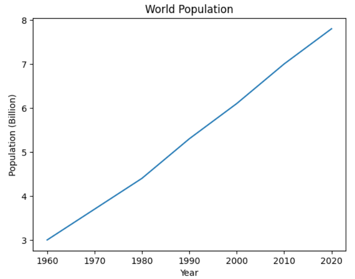
Although you've created a simple chart for demonstration purposes, you can further customize your chart any way you like using the capabilities of Matplotlib. After all, your notebook is using the same Matplotlib library that you may already be familiar with from your other programming projects.
Note
If you're using a function or method inside a Jupyter Notebook, then you can find information about it using the Shift+Tab keys. This will display its docstring content, if it has any. You can try this out by typing plt.title( followed by Shift+Tab.
Suppose you now decide that you no longer want to analyze all the data. Instead, you're interested in population data from 1980 onwards. All you need to do is update your data and rerun the cells.
Go ahead and update the original cell with the code shown below. You can comment out the original data just in case you want to return to it later:
# decades = [1960, 1970, 1980, 1990, 2000, 2010, 2020]

# World population (billions)
# population = [3, 3.7, 4.4, 5.3, 6.1, 7.0, 7.8]

decades = [1980, 1990, 2000, 2010, 2020]
population = [4.4, 5.3, 6.1, 7.0, 7.8]
Once you've made your changes, rerun the cell to update the content of the decades and population list variables. Then, to update the chart, you rerun the cell containing the chart code. With this, you've updated your chart, and it should now look like this:
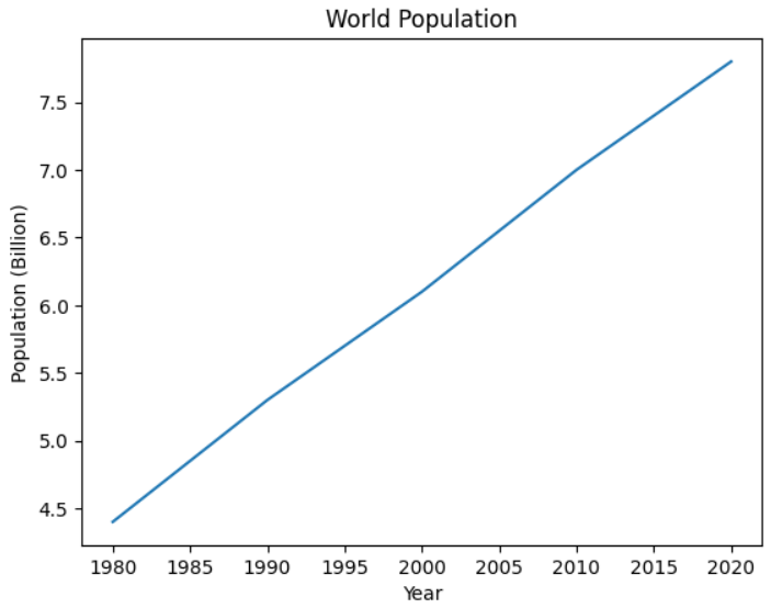
As you can see, only the years 1980 through 2020 are now displayed in your chart.
Note
You may also see a third cell type named raw. Anything that you type into these cells stays exactly the same as you originally typed it. You can't apply any formatting to it. You'd use these cells for typing data in common formats such as LaTeX source. These cells can, for example, be rendered by passing them to a TeX program.
Earlier you learned that JupyterLab contains features that enhance Jupyter Notebook. It's now time for you to see this in action.
Working With Multiple Notebooks
Next you'll learn how JupyterLab helps you work with multiple notebooks. To do this, of course, you'll need to create another notebook.
Keep your Population Data notebook open and open a second one. To do this, click the New Launcher ‘+' tab. Now launch another notebook by clicking the Python 3 icon under the Notebook heading. A second notebook will launch in its own tab. Right-click this tab and rename the notebook Population Changes:
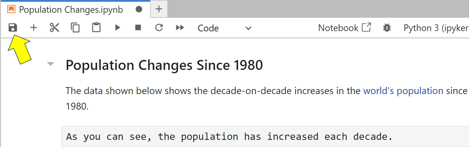
As you can see, the notebook tabs are placed beside each other. To keep things looking professional, you might like to add some Markdown explaining a little about the intended content of your Population Changes notebook:
---

## Population Changes Since 1980

The data shown below shows the decade-on-decade increases in the
[world's population](https://worldometers.info/world-population/world-population-by-year/)
since 1980.
Again, don't forget to run the Markdown cell using Shift+Enter to render it into the cell.
Although the current notebook arrangement makes it easy to flip between them by clicking their tabs, suppose you wanted to use this second notebook to analyze your world population data. The first thing you'd need to do is add in the population data from your Population Data workbook. You could, of course, copy and paste, but JupyterLab allows you to drag cells directly between different notebooks, provided you can see them both simultaneously:
To display notebooks side by side, you dragged the tab of the Population Changes notebook down and to the right of the Population Data notebook. When you released your mouse, both workbooks became viewable.
Then, to copy the cells between notebooks, you selected the cell containing the decades and population lists in Population Data. You know you've selected it when a blue vertical bar appears to the right of the cell.
Finally, you grabbed the margin area as shown and dragged it across onto Population Changes before dropping it. You used the fine blue horizontal line that appeared as a placement guide.
Note
If you've moved the cell into the wrong place, select it and drag it vertically to where you want it to go. Also, if you want to move the notebook back to where it was, drag the Population Changes tab back up and next to the Population Data tab where it originally was.
Adding a Python Library Into a Notebook
Next, you'll analyze the Population Changes notebook. To do this, you need to add some more code and import the pandas library.
In a code cell immediately below the one that you just copied across, add in the following code:
def calculate_differences(data_set):
    differences = [0]
    for index in range(1, len(data_set)):
        differences.append(round(data_set[index] - data_set[index - 1], 1))
    return differences

population_change = calculate_differences(population)
Your calculate_differences() function accepts a list of numbers and calculates the differences between each of its elements. These differences are returned as a separate list. The final line of code calls the function and stores the returned list when you run the cell. Nothing will be displayed.
Before you go any further, make sure to run this cell to ensure its content is known to the underlying kernel.
Next you'll create a pandas DataFrame. Having your data in a pandas DataFrame allows you to perform lots of data analysis on it. Here you'll settle for a neat table containing the data.
pandas is another module that's not part of the native Python language, so you'll need to install it. To do so, add a new code cell and use !python -m pip install pandas. Run the cell, and pandas will install. Check the final line of the output to make sure there were no installation errors. You can then delete the output of the pip install command by selecting its cell and sending it to trash.
Note
The pandas module has actually been installed into the underlying Python programming environment or virtual environment that's driving each of your notebooks. This means that instead of rerunning the pip command in other notebooks, you only need to import pandas. Also, the next time you restart JupyterLab, pandas will still be there for you.
Once you've successfully installed pandas, you can use it to analyze your data any way you wish. Here you only want a DataFrame, so add the following code into a code cell in your notebook:
import pandas as pd

zipped = list(zip(decades, population, population_change))
columns=["Decade", "Population(Bn)", "Change"]
population_df = pd.DataFrame(zipped, columns=columns)

print(population_df)
To use the pandas module that you just installed, you must import it. You then use Python's built-in zip function to iterate over each of your lists in parallel and produce a collection of tuples with an item from each one. You then pass that collection into the pandas DataFrame constructor to produce a DataFrame. In addition, you specify the columns of the DataFrame using the columns parameter.
As you can see when you run the cell, the DataFrame displays as a neat table:
| Decade | Population(Bn) | Change | |
|---|---|---|---|
| 0 | 1980 | 4.4 | 0.0 |
| 1 | 1990 | 5.3 | 0.9 |
| 2 | 2000 | 6.1 | 0.8 |
| 3 | 2010 | 7.0 | 0.9 |
| 4 | 2020 | 7.8 | 0.8 |
Did you know that the world's population is increasing at a nearly constant rate each decade? Oh, the things you learn from Real Python tutorials!
Looking at Views
If you have a long file, you may need to scroll down to view what you're interested in. To overcome this, JupyterLab allows you to create multiple synchronized views of your files. When you create a new view on a file such as a notebook, you're creating a new interface for accessing it. Each view allows you to look at separate parts of your file at the same time. What's more, if you change a notebook, its view updates as well.
Suppose you want to view your Matplotlib chart outside of its notebook. To do this, you create a new view of your chart in its own tab. However, the chart will still be linked to the underlying notebook code. If you change the chart's data in the notebook, then you'll update the chart in both the notebook and the view. This is very useful if your notebook is long and you want to see different parts of it at the same time.
Note: While you can't create views of Markdown cells, you can work around this by creating a view of an entire notebook. To do this, right-click on the tab of the workbook that you wish to create a view on and choose New View for Notebook. Your new view will appear in a separate tab. You can then scroll around the view independently of the original notebook.
Select your Population Data notebook and then the cell containing the Matplotlib code:
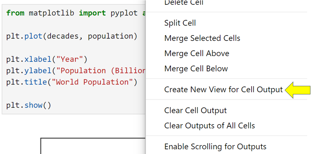
Now right-click on the cell or the existing chart and select Create New View for Cell Output. A new view tab will appear below the notebook. You can move the position of the view around the screen to wherever you wish by dragging and dropping its tab. The view will always display the same content regardless of which cells you're looking at in its underlying notebook:
As you can see, the new view appears immediately below the notebook that it's a view of. Feel free to change the data contained in your population data notebook and rerun its cell as well as the cell containing the chart. In addition to updating the chart in the notebook, this will also update it in the view.
If you close the notebook, you'll close the view. Unlike notebooks, views aren't saved. To close the view alone, simply close it by clicking the X on its tab.
Note
Views are most commonly associated with Jupyter Notebooks, but you can actually create them on any file type available within JupyterLab. As an example, you could create two views on a long PDF file that allow you to see both its first and last pages. Also, because all views on a file are looking at the same file, any changes that you make through one view will reflect in the other views.
Of course, creating multiple views when combined with opening multiple files can be very useful, but it would be tiresome having to open everything up again each time you restart JupyterLab. Fortunately, you don't actually have to, as you'll see next.
Working With Workspaces
A JupyterLab workspace is a saved layout of its various components, such as open notebooks and terminals. By default, JupyterLab saves changes to your layout automatically. This allows you to continue with the same layout that you had when you last closed it. You'll find this very useful if you perform your analysis over many sessions.
If you're working on multiple projects that all need their own sets of files or other components opened simultaneously, you can save their layout as a custom workspace so that you can quickly return to it again later.
A workspace is a JSON file containing information about the files it contains and their layout on-screen. This means that if you delete the workspace file, you won't delete any files that it references.
It's possible to save the layout of the contents of a JupyterLab session, including its views. To do this, you save the workspace. First of all, make sure you've saved everything. You can do this quickly by choosing the File → Save All menu option. To save the layout, select File → Save Current Workspace As, and then give it a name such as population_analysis.jupyterlab-workspace. This will add a workspace layout file to the file browser:
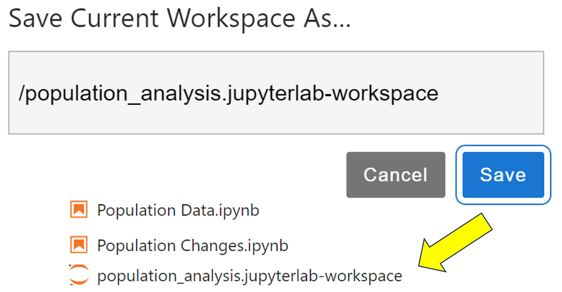
The next time you open JupyterLab, it'll display everything the way it was when you last closed the program because it automatically updates workspaces as you change them. To return to a saved workspace, double-click on its file from the browser, and everything will reset to the way it was when you last saved it. When you make changes to a layout, choose File → Save Current Workspace to update your saved workspace.
Sharing Code Between Notebooks
If you need to perform lots of analysis in a notebook, there's a danger that your notebook will become long and difficult to work with. Instead of creating a single large notebook, it'd be better to split your analysis down into separate notebooks. One way would be to duplicate your data, but this creates data management issues whenever your data changes. Fortunately, JupyterLab allows you to share data from one notebook with others.
Earlier you learned that the kernel is responsible for passing the code from a notebook to a console for running. Once the code has finished, the kernel returns its output back to your Jupyter Notebook for display. So, the kernel provides access to any data or functions that your program uses. By linking additional notebooks to the kernel of a notebook, its content becomes available to those additional notebooks.
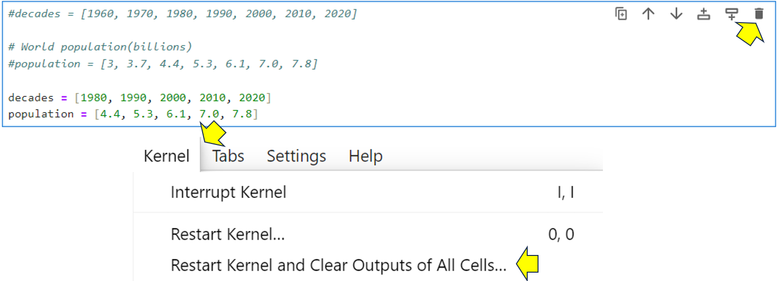
Locate the cell in your Population Changes notebook that contains the Python population data lists that you copied earlier and delete it by clicking the trash can icon in the top-right corner of the cell. At this point, the notebook's kernel will still hold the data. To fix this, choose Kernel → Restart Kernel → Clear Outputs of All Cells from the menu. This will reset your notebook. It'll still contain its content, but not its output:
Now rerun the Population Changes cell that contains your calculate_differences() code and watch as it fails:
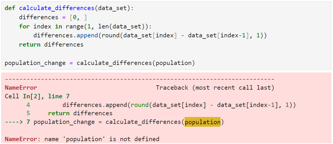
As you can see from the traceback, your code has raised a NameError. This has happened because your code can no longer find the population list that it needs. That's because the list was removed from the kernel when you cleared it and is now unknown to your code.
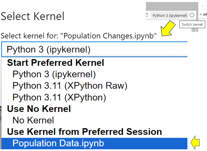
To deal with this and make sure you use the same data source as your original Population Data notebook, you must share the kernel that Population Data is using with Population Changes. You can do this by selecting the Population Changes notebook and clicking the Switch kernel button in its top-right corner. From the dropdown, select the Population Data kernel as shown:
Now when you rerun all the cells in Population Changes, everything works as before. The population list is available once more.
If you like, you can experiment by changing the data in your Population Data notebook and rerunning both notebooks again. If you do, just remember to rerun the cell where you changed your data to update the shared kernel.
Checkpointing Your Notebook
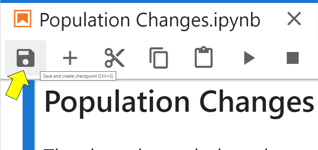
When you work with a Jupyter Notebook, it automatically saves any changes that you make. However, it's also possible to manually save a notebook. In the language of JupyterLab, this is called checkpointing, and you do it using Ctrl+S in Windows and Linux or Cmd+S in macOS. You can also click the Save and create checkpoint icon as shown:
When you first create a new notebook file, JupyterLab creates a file with an .ipynb file extension. In addition, it also creates a second .ipynb checkpoint file. This starts with the same name as the original notebook file, only with -checkpoint appended to it. This checkpoint file gets placed inside a hidden folder named .ipynb_checkpoints in the same folder as your original notebook.
By default, the initial notebook file and its checkpoint will be blank. When you add content to your notebook, the original notebook file gets automatically saved every two minutes. The checkpoint file remains untouched.
If you want to update the checkpoint file as well as the notebook file, then you do so by performing a manual save using Ctrl+S in Windows or Linux, Cmd+S in macOS, or File → Save Notebook from the menu. Doing this overwrites your previous checkpoint. If you then make changes to your notebook, JupyterLab autosaves them every two minutes, but again, the checkpoint is untouched.
Although autosaving is useful, it does mean that any incorrect changes that you make are also automatically saved. This is where checkpoints can help you. It's possible to roll your notebook back to the last checkpoint by using File → Revert Notebook to Checkpoint….
To test this, add a new raw cell below the last cell of your Population Changes notebook and enter the text As you can see, the population has increased each decade. A raw cell contains completely unformatted and unformattable text. Now manually save the notebook to update its checkpoint:
Next double-click on your raw cell to edit it, and change this cell to read As you can see, the population has decreased slightly each decade. Wait at least two minutes then close your notebook without saving it, and shut down the server. Next restart the JupyterLab server once more. When you reopen your notebook, these changes should still be in it. If not, you haven't waited long enough. Try again, but this time be more patient.
Now you realize you wish you hadn't made this change. To revert back, select the File → Revert Notebook to Checkpoint menu option. When you're asked to confirm, click the red Revert button. Now take a look at the cell that you changed:
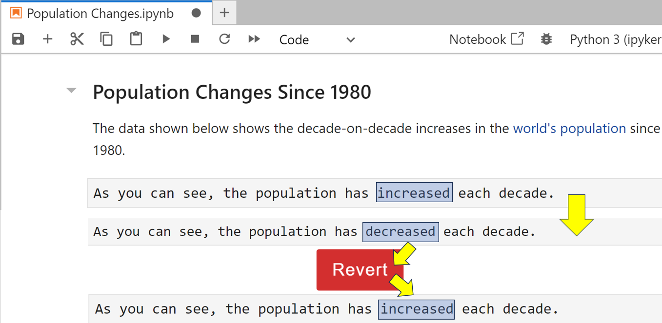
As you can see, decreased has rolled back to increased. Thankfully, your invalid changes are gone.
The checkpointing feature within JupyterLab is fairly primitive. In essence, it offers you the capability to revert to the last manually saved version. You can only revert back to the last checkpoint, and once you've done so, you can't roll back any further or even roll forward again. Before you perform a manual save, make sure your changes are safe for permanent saving. You can't undo this if they're not.
If you find that you're making changes to your notebooks and want to retain earlier versions, the only way within JupyterLab is to create multiple versions of each file by using File → Save Notebook As and giving each a slightly different filename. Obviously, this could still leave you with version control issues.
Note
Although you may be disappointed that JupyterLab's support for version management is somewhat primitive, there's a package called nbdime that can improve things. It provides tools that allow you to highlight differences between, or merge together, two notebooks. The package name, nbdime, is in fact short for notebook diff and merge.
Before you move on to some of the other features of JupyterLab, you'll finish off by learning how to debug notebooks. This is something that you may not have seen, even if you've used Jupyter Notebooks before.
Debugging Your Notebook
JupyterLab uses the integrated debugger found within later versions of Jupyter Notebook. The integrated debugger allows you to perform common debugging tasks such as running code one line at a time to verify that it's working the way you expect it to. You can also monitor the values of variables to make sure they contain what you expect them to.
As an example, you'll run the debugger against your calculate_differences() function in your Population Changes notebook. Although this function works just fine, you'll still use it to gain experience in operating the debugger.
To enable the integrated debugger inside your notebook, click the small bug icon in the top-right corner. The bug will turn orange to show that the integrated debugger is switched on:
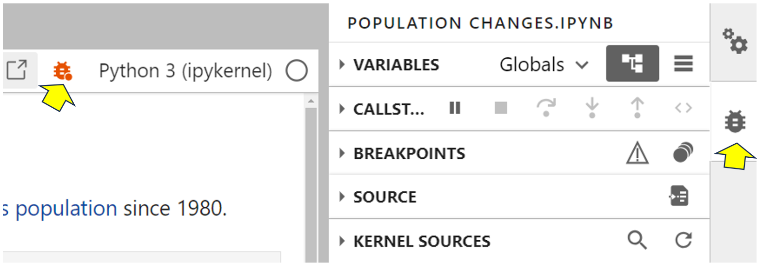
With the debugger on, the debugger tab will be selected at the right of your screen. This tells you what your code is doing while it runs. The debugger contains various sections, including Variables, Callstack, and Breakpoints. Some of them will already be expanded, but they're all collapsed for convenience here. Also, with the debugger switched on, each code cell gets line numbers. You can use these for reference during debugging.
Start off by running all the cells in your notebook. The quickest way to do this is to choose Run → Run All Cells from the menu. This will allow you to learn how the debugger displays the notebook's variables.
Expand the variables section of the integrated debugger. Click the Table View icon, and you'll see the complete set of variables that your notebook's code uses, along with their current values:
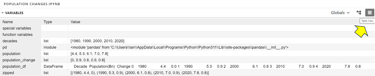
Take a moment to look through the information on display. You can see the content of the various lists, the DataFrame, and even the zipped list that you used to create the DataFrame. This screen is one of the most important when using the debugger.
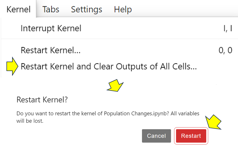
To see the debugger in action, you first of all clear everything from the notebook's memory. To do this, you need to select Kernel → Restart Kernel and Clear Outputs From All Cells, then click Restart:
This will clear all outputs and variables from the notebook. If you now look at the list of variables, then you'll see that you've cleared all of them. Each notebook has its own kernel, allowing you to clear each one independently of the others. In restarting the kernel, you've also disabled debugging.
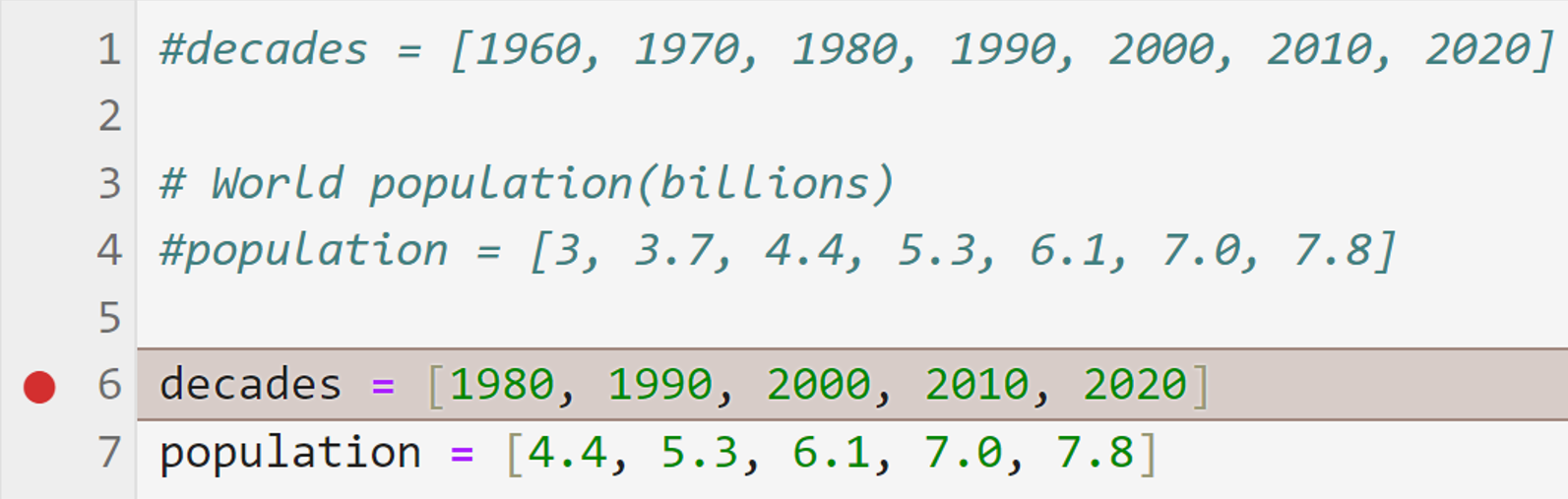
Next, to see how to use the integrated debugger, you'll debug your code. To begin with, enable the debugger once more and arrange the Variables, Callstack, and Breakpoints sections as shown. Also set a breakpoint by clicking on the margin next to your decades list as shown below:
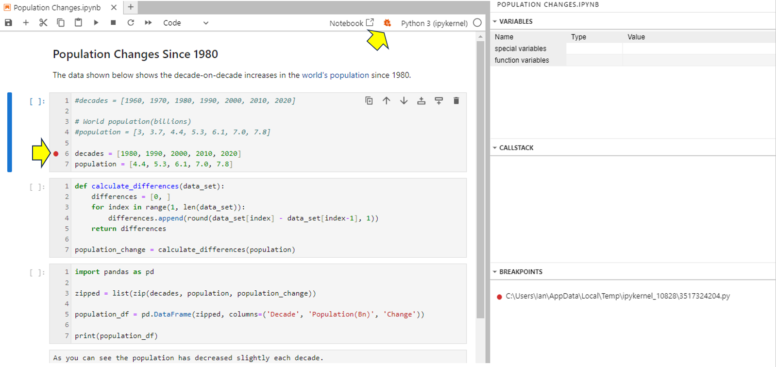
You'll see the breakpoint added to the Breakpoints section of the debugger. A small red dot appears next to the line to indicate that it has a breakpoint. Your code will run normally up to the breakpoint, and then it'll enter debug mode. Once in debug mode, you can run the code at your own pace to monitor it. In this case, your entire code will run in debug mode because you've created a breakpoint at its first line.
To start debugging, make sure debugging is switched on, and then choose Run → Run All Cells from the menu. Your code will stop at the first breakpoint that it encounters, which will be highlighted:
Your notebook's code has now paused processing and is awaiting your instruction on how it should proceed next. The choices are displayed visually in the bar above the callstack section of the debug window:
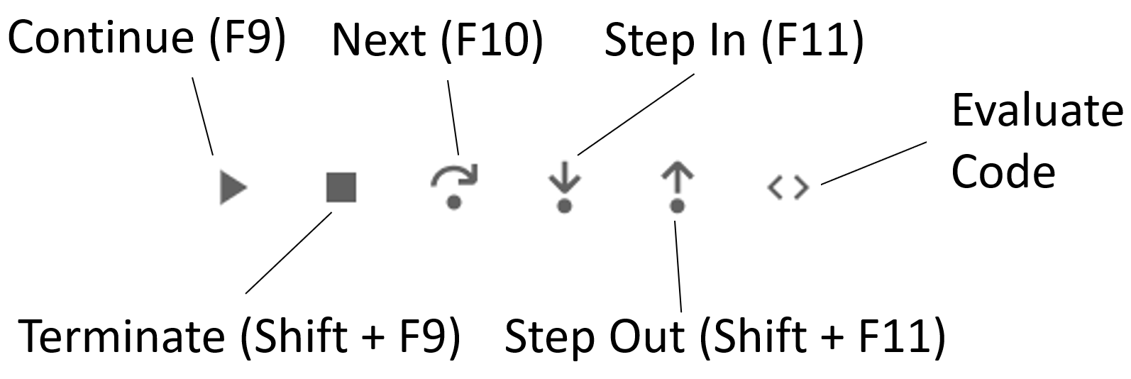
When you click on each of these icons, the program behaves slightly differently. As a starting point, consider the first three options:
- Continue will cause the rest of your code in the cell to run at normal speed, unless you've inserted a second breakpoint, in which case it'll run normally to that breakpoint and then reenter debug mode.
- Terminate will immediately stop the code in the cell from running.
- Next will run the next line of code and then pause to await your further instruction. This is how you run an entire program one line at a time, automatically updating the variables section as each variable is populated. This is one of the most common operations that you use when debugging code.
To understand the debugger better, with the notebook still awaiting you instructions, select Next or tap F10. The code will progress to the next line and pause once more:
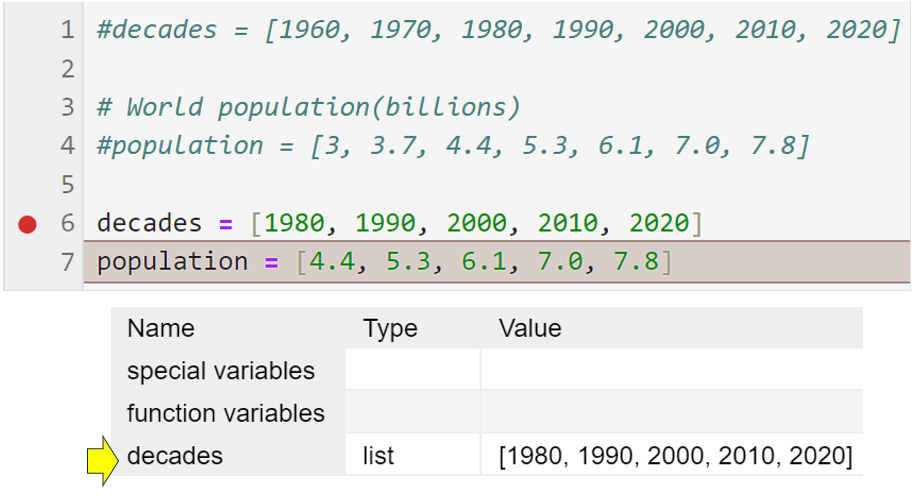
Pay particular attention to the variables section on the right, and you'll see that the decades variable now has some data assigned to it. This has happened because line 6 ran successfully. By noting this information, you can verify that this line of code is working as expected.
Now tap F10 once more. As you might expect, the population variable now contains data. The program has moved to the top of the next cell containing your calculate_differences() function, and then it stops.
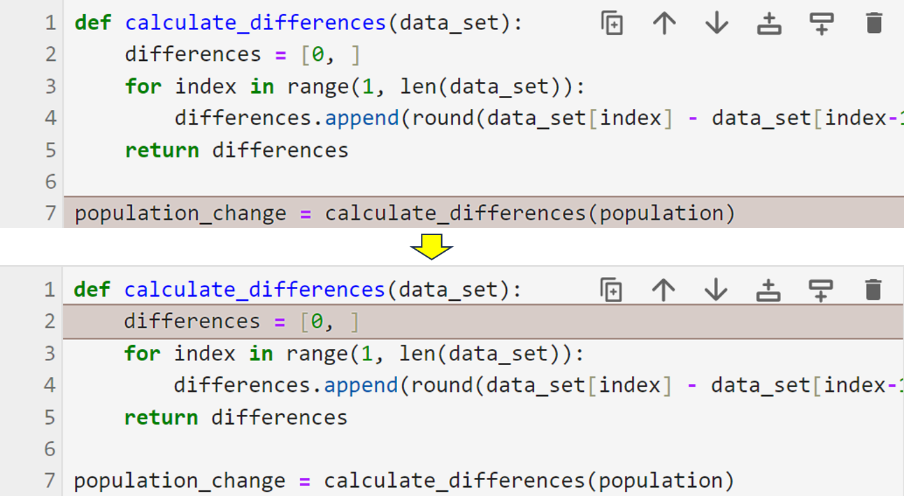
Now tap F10 once more, and control moves to the first line beyond the function. This is because only the line containing the function header has been processed. The function body can only run when your code calls it. In processing the header, your code now knows the function exists.
At this point, you have a choice to make. If you tap F10 again, you assign the population_variable its data, and the program ends. You may have expected the debugger to enter your calculate_differences() function and run through it. In fact, the function did run, but it did so at full speed. Selecting F10 runs a complete line of code at full speed, including any calls to functions. This is why the Next icon has an arrow jumping over a dot.
You can verify that the function has indeed run because if you look at the list of variables, you'll see that population_change now has content:
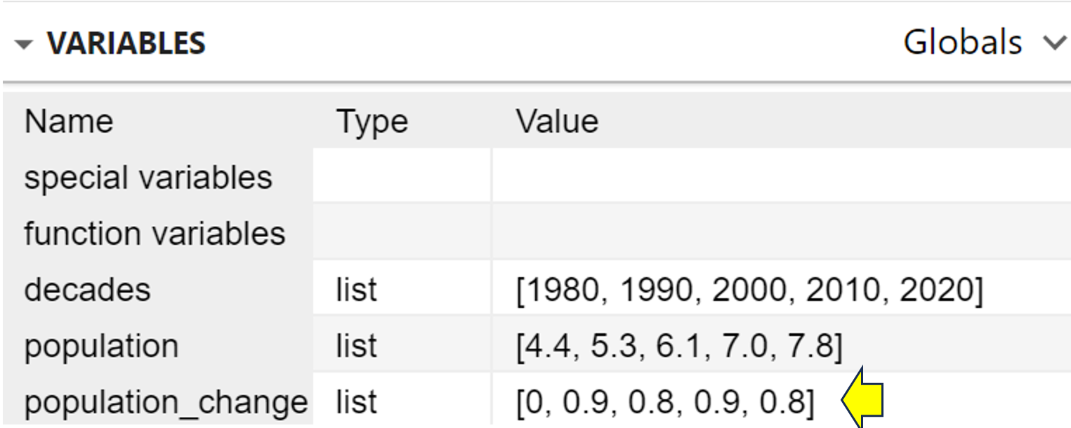
As you can see, the population changes now show up in the population_change list.
Of course, there will be times when you need to run the debugger through the function code. To do this, tap the Terminate button in the callstack section or use Shift+F9. This will stop the debugger. Now restart the debugger and repeat the previous instructions until your notebook has stopped at the function call line. You'll have tapped F10 three times to get there.
This time, instead of using F10, tap F11 or choose the Step In option in the callstack section instead. As its name and icon suggest, this will move into the code by entering the function's body:
As you can see, the debugger now allows you to step through the function's code, and it has stopped at the first line of the function's body. Notice that the data_set variable, which only exists within the function, now contains data. Also, the callstack tells you that program control has left line 7 in the main module and entered line 2, which is in the calculate_differences() function. This information allows you to monitor the program's flow.
Tap F10 a few times more until you've completed at least one iteration of the for loop. Keep an eye on the variables section, and you'll see the variables change as the loop iterates. Again, you could run through the entire function one line at a time if you wanted to.
Once you're satisfied that your function is working correctly, you can tap the Step Out button or use Shift+F11 to run the remainder of the function at normal speed and jump back to line 7, where you called it. Tap F10 once more, and this final line of code will run, completing the cell.
If you have the debugger switched on and don't set any breakpoints, then running the code causes it to to run at normal speed. However, the debug window will still contain the value of every variable. This can be useful if you want to see what values your program is storing without printing.
Finally, you can remove an individual breakpoint by clicking on its red circle. The quickest way to switch all breakpoints off is by clicking the red bug symbol to switch debugging off and then clicking it again to switch debugging back on again.
While notebooks are by far the most commonly used component of JupyterLab, they're not the only one. You'll now turn your attention to some of its other interesting features.