DBSCAN Clustering
DBSCAN Clustering 관련

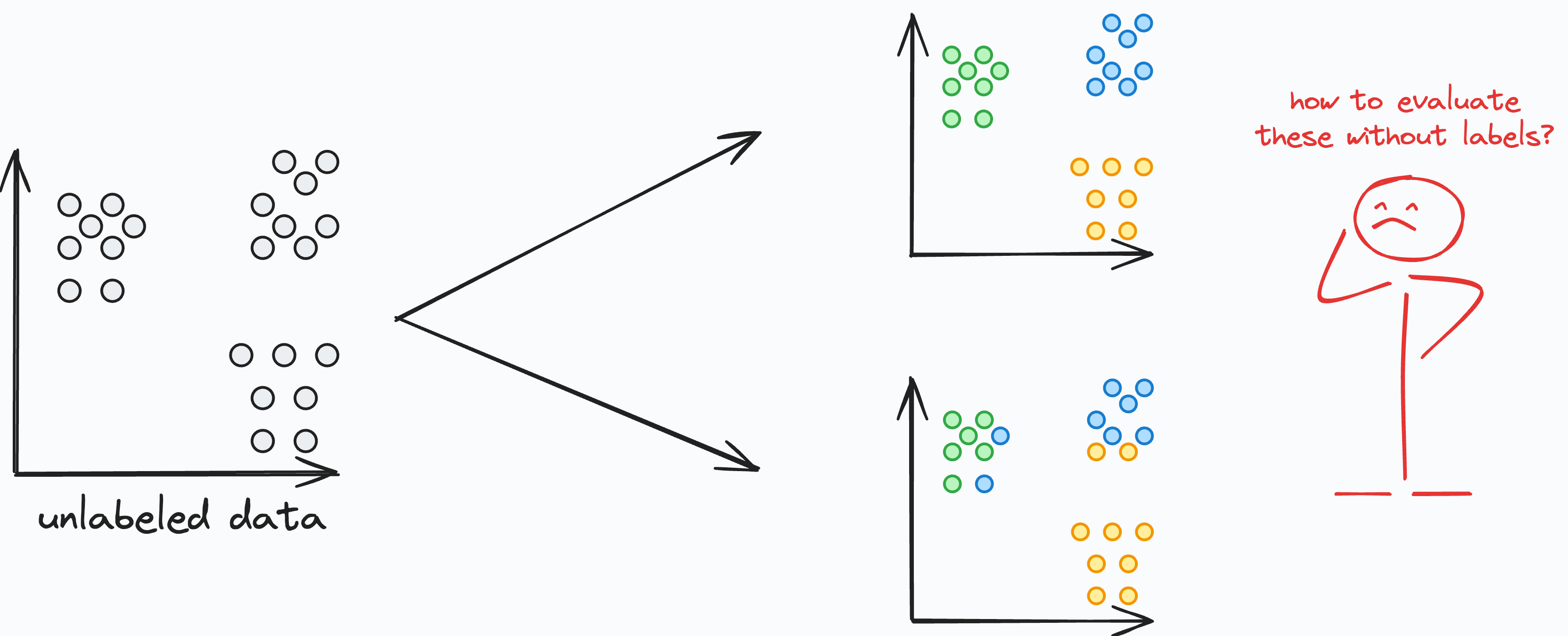
DBSCAN (Density-Based Spatial Clustering of Applications with Noise) is an unsupervised learning algorithm used for clustering analysis. It’s particularly effective in identifying clusters of arbitrary shape and handling noisy data.
Unlike K-Means or Hierarchical clustering, DBSCAN does not require specifying the number of clusters in advance. Instead, it defines clusters based on density and connectivity within the data.
How DBSCAN Works
Density-Based Clustering
DBSCAN groups data points together that are in close proximity to each other and have a sufficient number of nearby neighbors. It identifies dense regions of data points as clusters and separates sparse regions as noise.
Core Points, Border Points, and Noise Points
DBSCAN categorizes data points into three types: Core Points, Border Points, and Noise Points.
- Core Points: Data points with a minimum number of neighboring points (defined by the
min_samplesparameter) within a specified distance (defined by theepsparameter). - Border Points: Data points that are within the
epsdistance of a Core Point but do not have enough neighboring points to be considered Core Points. - Noise Points: Data points that are neither Core Points nor Border Points.
Reachability and Connectivity
DBSCAN uses the notions of reachability and connectivity to define clusters. A data point is considered reachable from another data point if there is a path of Core Points that connects them. If two data points are reachable, they belong to the same cluster.
Cluster Growth
DBSCAN starts with an arbitrary data point and expands the cluster by examining its neighbors and their neighbors, forming a connected group of data points.
Benefits of DBSCAN Clustering:
- Ability to detect complex structures: DBSCAN can discover clusters of various shapes and sizes, making it well-suited for datasets with non-linear relationships or irregular patterns.
- Robust to noise: DBSCAN handles noisy data effectively by categorizing noise points separately from clusters.
- Automatic determination of cluster numbers: DBSCAN does not require specifying the number of clusters in advance, making it more convenient and adaptable to different datasets.
- Scaling to large datasets: DBSCAN’s time complexity is relatively low compared to some other clustering algorithms, allowing it to scale well to large datasets.
In the next section, we will delve into the implementation of the DBSCAN algorithm in Python, providing step-by-step guidance and examples.
DBSCAN Clustering: Python Implementation
In this section, I’ll guide you through how to implement DBSCAN using Python.
Key Steps for DBSCAN Clustering
- Prepare the data: Before applying DBSCAN, it is important to preprocess your data. This includes handling missing values, normalizing features, and selecting the appropriate distance metric.
- Define the parameters: DBSCAN requires two main parameters: epsilon (ε) and minimum points (MinPts). Epsilon determines the maximum distance between two points to consider them as neighbors, and MinPts specifies the minimum number of points required to form a dense region.
- Perform density-based clustering: DBSCAN starts by randomly selecting a data point and identifying its neighbors within the specified epsilon distance. If the number of neighbors exceeds the MinPts threshold, a new cluster is formed. The algorithm expands this cluster by iteratively adding new points until no more points can be reached.
- Perform noise detection: Points that do not belong to any cluster are considered as noise or outliers. These points are not assigned to any cluster and can be critical in identifying anomalies within the data.
To perform DBSCAN clustering in Python, we can use the scikit-learn library. The first step is to import the necessary libraries and load the dataset we want to cluster. Then, we can create an instance of the DBSCAN class and set the epsilon (eps) and minimum number of samples (min_samples) parameters.
Here is a sample code snippet to get you started:
import numpy as np
import matplotlib.pyplot as plt
from sklearn.datasets import make_moons
from sklearn.cluster import DBSCAN

# Generate some sample data
X, _ = make_moons(n_samples=500, noise=0.05, random_state=0)

# Apply DBSCAN
db = DBSCAN(eps=0.3, min_samples=5, metric='euclidean')
y_db = db.fit_predict(X)

Remember to replace X with your actual data set. You can adjust the eps and min_samples parameters to get different clustering results. The eps parameter is the maximum distance between two samples for one to be considered as in the neighborhood of the other. The min_samples is the number of samples (or total weight) in a neighborhood for a point to be considered as a core point.
DBSCAN offers various advantages over other clustering algorithms, like not requiring the number of clusters to be predefined. This makes it suitable for data sets with an unknown number of clusters. DBSCAN is also capable of identifying clusters of varying shapes and sizes, making it more flexible in capturing complex structures.
But DBSCAN may struggle with varying densities in data sets and can be sensitive to the choice of epsilon and minimum points parameters. It is crucial to fine-tune these parameters to obtain optimal clustering results.
By implementing DBSCAN in Python, you can leverage this powerful clustering algorithm to uncover meaningful patterns and structures in your data.
Before we explore the differences between DBSCAN and other clustering techniques, let’s take a closer look at the key parameters that influence DBSCAN’s performance and results.
Understanding Key Parameters in DBSCAN
The eps (epsilon) parameter defines the maximum distance between two points for one to be considered as a neighbor of the other. This means that points within this radius of a core point belong to the same cluster. Choosing an appropriate eps value is crucial, as a very small eps may lead to too many small clusters, while a very large eps could merge distinct clusters into one.
The min_samples parameter determines the minimum number of data points required to form a dense region. If a point has at least min_samples neighbors within the eps radius, it is classified as a core point. If a point falls within the eps radius of a core point but does not meet the min_samples threshold itself, it is classified as a border point. Any point that is neither a core point nor a border point is labeled as noise or an outlier.
How DBSCAN Groups Data Points
DBSCAN operates by identifying core points and expanding clusters around them. It groups together closely packed points (or clusters) based on density and marks low-density points as outliers (or noise). The process follows these steps:
- Select an unvisited point and check if it has at least
min_samplesneighbors within theepsradius. - If it does, this point becomes a core point, and a new cluster is formed around it.
- Expand the cluster by adding all directly reachable points within
eps. If any of these points are also core points, their neighbors are added as well. - Continue expanding until no more points meet the density criteria.
- Move to the next unvisited point and repeat the process.
- Classify remaining points as border points (part of a cluster but not core points) or noise (outliers that do not belong to any cluster).
Example Implementation of DBSCAN
In this implementation:
eps=0.3: Defines how close points should be to be considered neighbors.min_samples=5: Sets the minimum number of points required to form a dense region.fit_predict(X): Assigns a cluster label to each data point.
After applying DBSCAN, the data points are assigned labels. If two points belong to the same cluster, they will have the same label in y_db. Points identified as outliers will be labeled as -1 and remain unclustered.
The resulting scatter plot visually represents how DBSCAN has identified two moon-shaped clusters. Unlike K-Means, which assumes spherical clusters, DBSCAN is able to detect arbitrary-shaped clusters effectively.
plt.scatter(X[y_db == 0, 0], X[y_db == 0, 1],
            c='lightblue', marker='o', s=40,
            edgecolor='black',
            label='cluster 1')
plt.scatter(X[y_db == 1, 0], X[y_db == 1, 1],
            c='red', marker='s', s=40,
            edgecolor='black',
            label='cluster 2')
plt.legend()
plt.show()

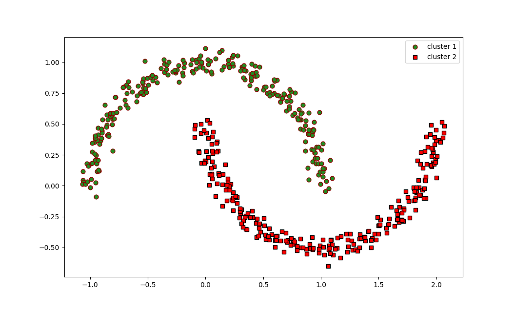
The resulting plot will show two moon-shaped clusters in green and red colors, demonstrating that DBSCAN successfully identified and separated the two interleaved half circles.